The following is a transcript of the presentation video, edited for clarity.
I’m going to be talking about more theory than models that so at least most of what I have to say is model-free, it doesn’t depend on which model you’re going to be using. However, I’m going to use a lot of symbols, and I’m going to try to make them so that they have some meaning. And I’m going to focus on outcomes. We’ve been talking about outcome measures, but we haven’t yet talked about how we use this to measure outcomes, the effects of what we’re doing. And so I want to look at it more from a theoretical point of view of what these models have to do and how you have to interpret them when you’re measuring outcomes.
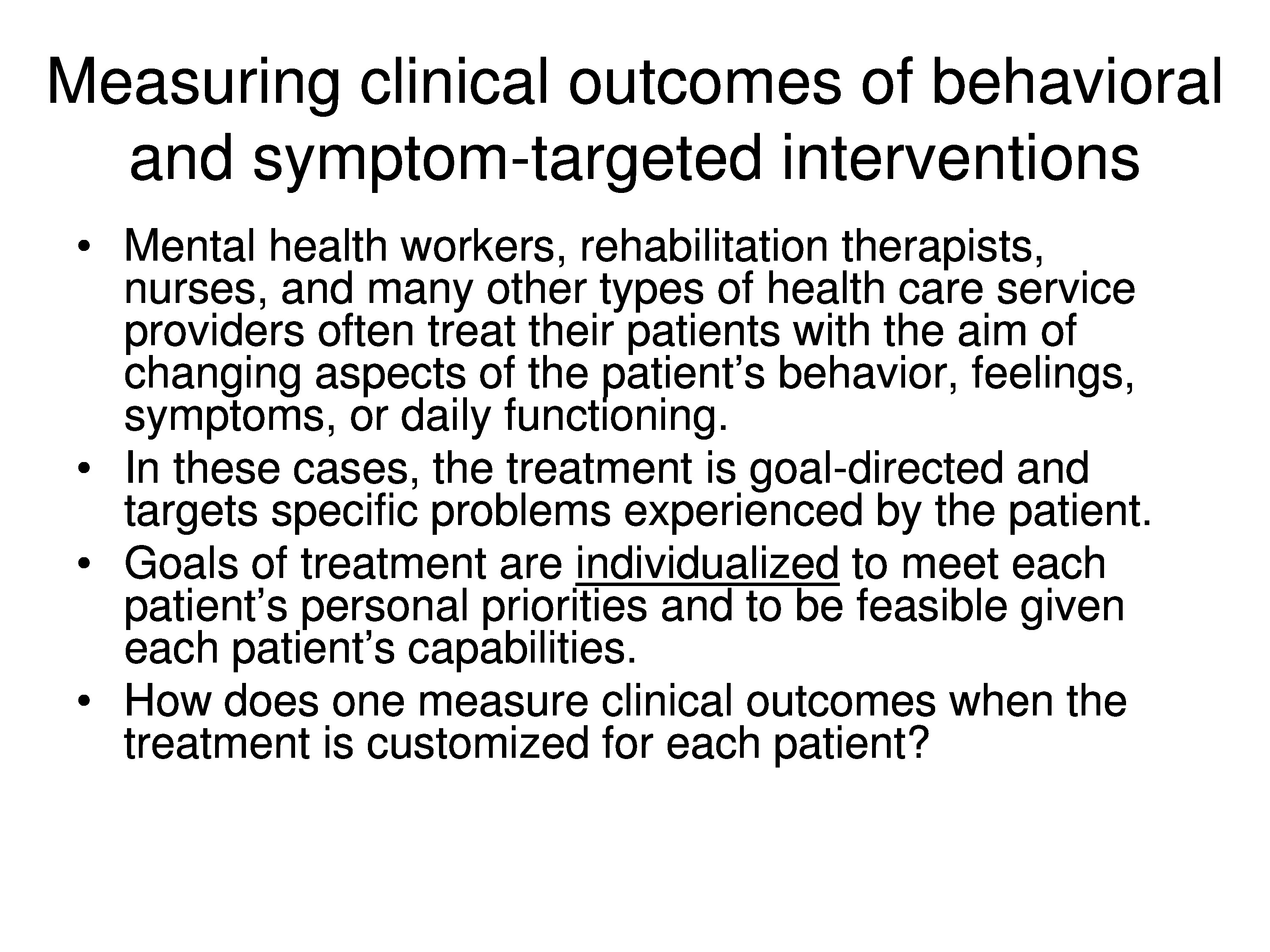
In measuring clinical outcomes of behavioral and symptom-targeted interventions we’re looking at changing aspects of patient’s behavior, feelings, symptoms, or daily functioning. And in these cases, the treatment is goal directed and targets specific problems that are experienced by the patient. The goals of treatment are highly individualized to meet each patient’s personal priorities and to be feasible given each patient’s capabilities.
The question is: How does one measure outcomes when the treatment is customized to each patient?
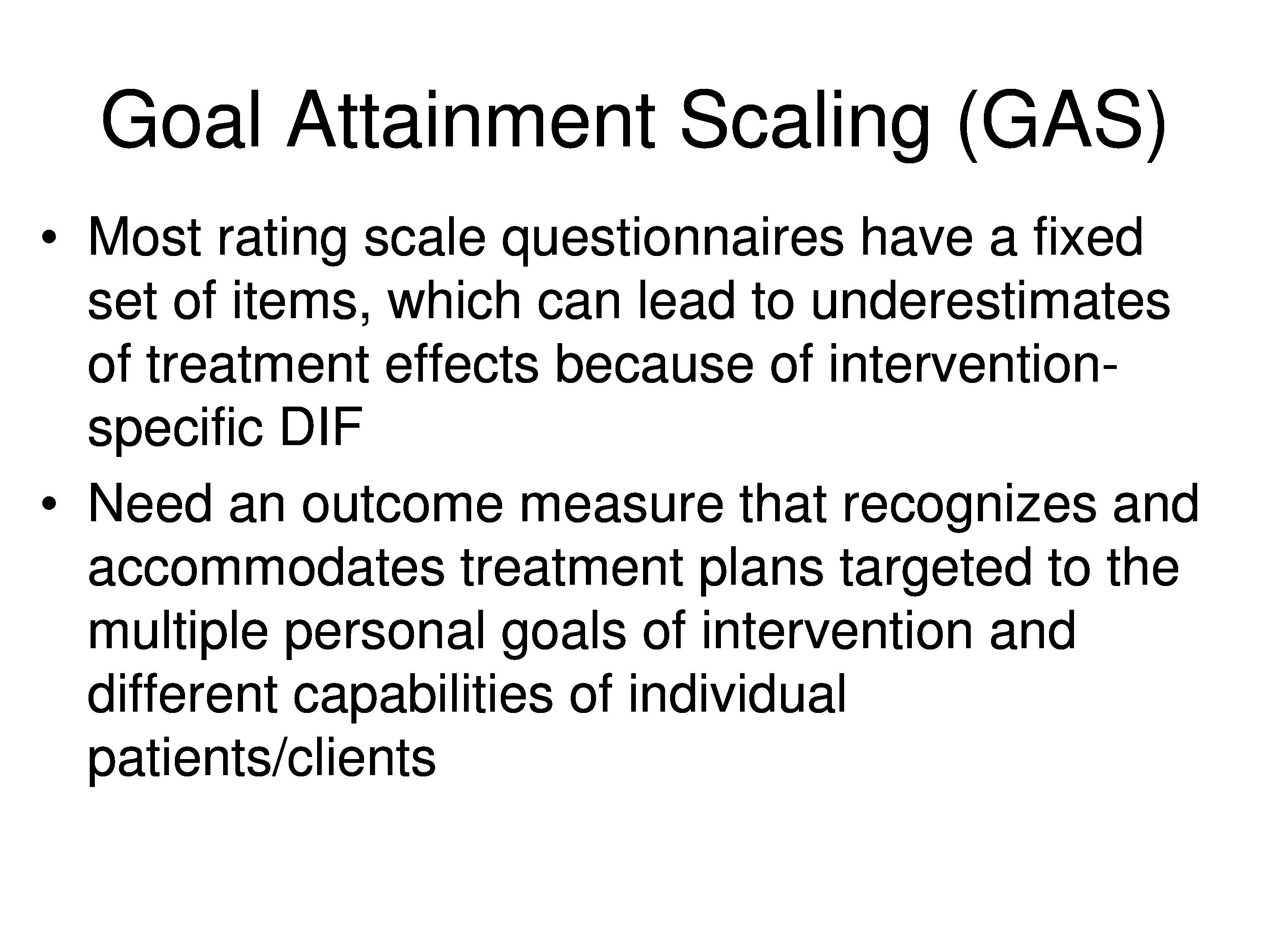
We need an outcome measure that recognizes and accommodates treatment plans targeted to the multiple personal goals of intervention and different capabilities of individual patients and clients. The goal attainment scale or GAS, which makes for a number of very clever slides, first developed in the late 1960s by Thomas Kiresuk, who is a clinical psychologist and his math-magician, Robert Sherman, to serve this need.
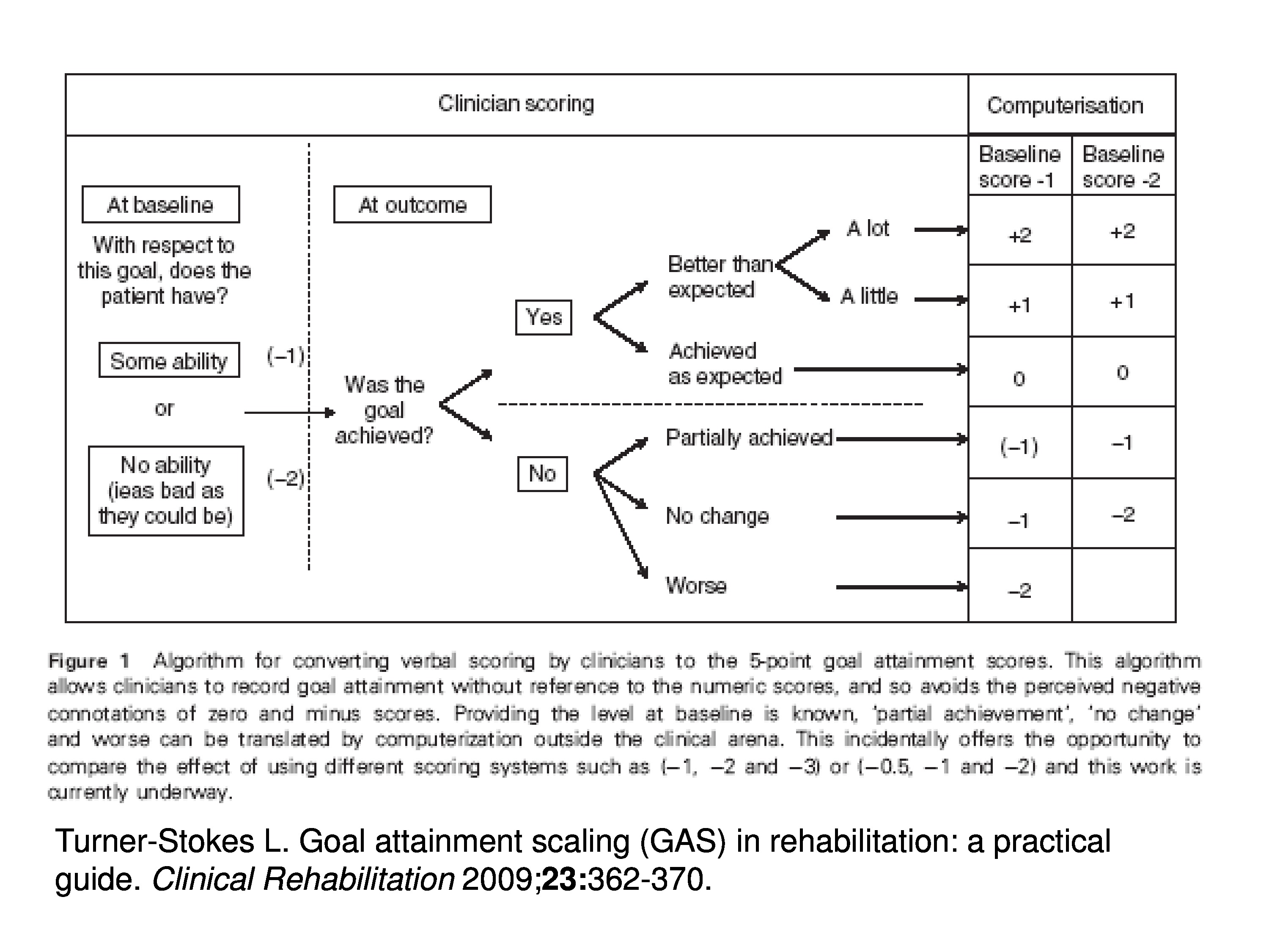
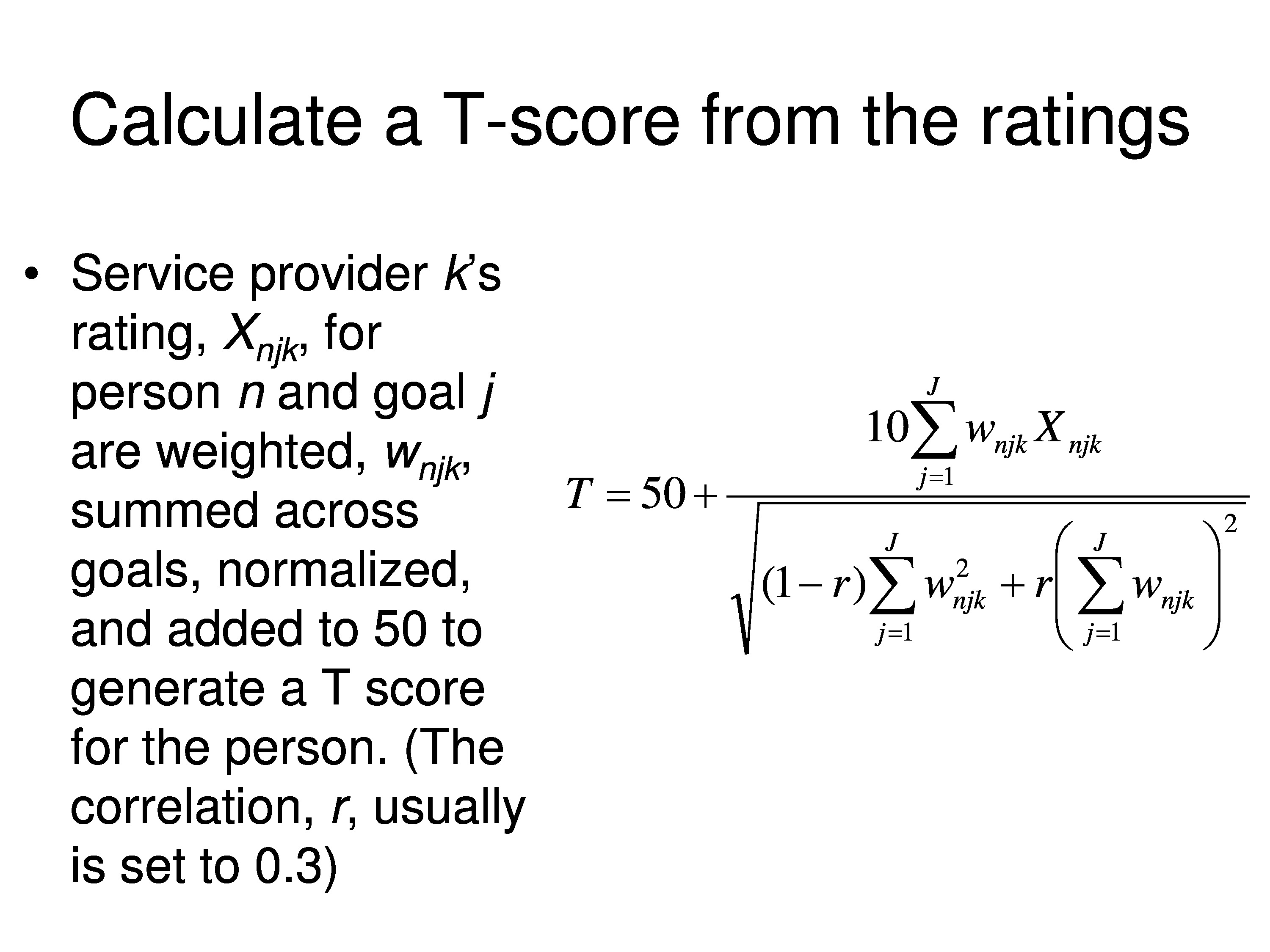
Goal attainment scaling, the way it’s implemented, basically, is that at baseline during the evaluation the clinician sets goals for the patient and then rates how far the patient is from the goal.
The goal would be at the origin of scale, it would be at zero. And rating might be, they have at the baseline which case they’d get a rating of zero or they’re at the goal at baseline, or they have some ability which case they’d be given a score of minus 1. Or they have no ability, things are as bad as they could be, they’d be given a score of minus 2.
Upon follow-up then they ask: Was the goal achieved? And if it was, then the rate above zero, it could be zero if it’s at the goal, it could be above zero if they did a little bit better than expected, and it would be plus 2 if they did a lot better than expected. Or they could lose ground. Or if the goal wasn’t achieved but they, maybe, made progress so it could be get closer to the goal but not achieve it and there would be ratings accordingly. So there’s just ordinal ratings that are assigned to distance from the goal, and it’s done on a goal-by-goal basis.
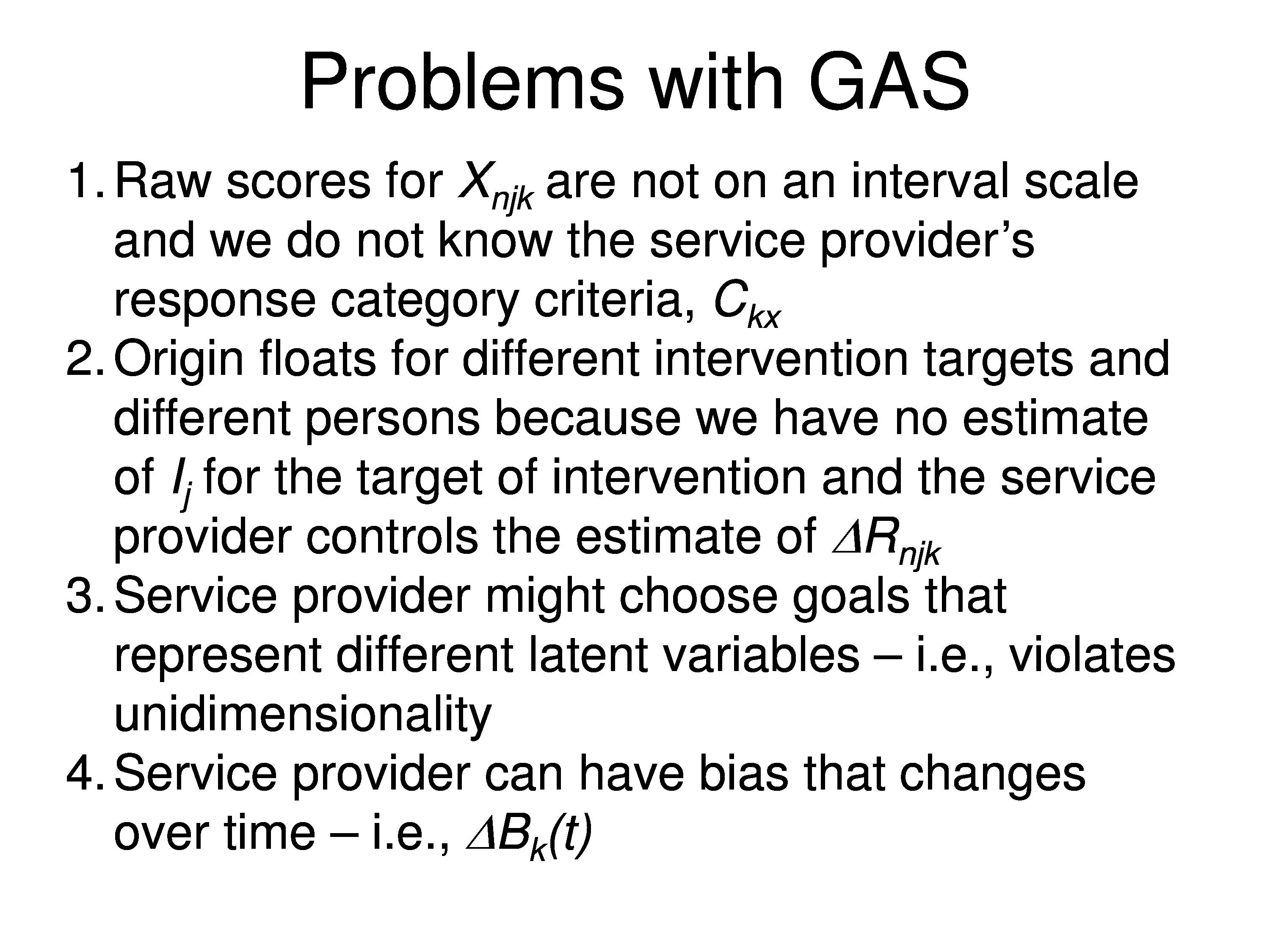
GAS relies on therapist ratings, which necessarily incorporate therapist’s specific biases. And the outcomes are scaled relative to the choice of goals in the rehabilitation plan.
A rating of zero means the patient is at the goal, but not all goals are the same, so the meanings of the scale changes across goals. Zero doesn’t mean the same thing for every goal.
So we need a theory that explicitly identifies all the relevant variables and then can be reduced to a valid measurement model.
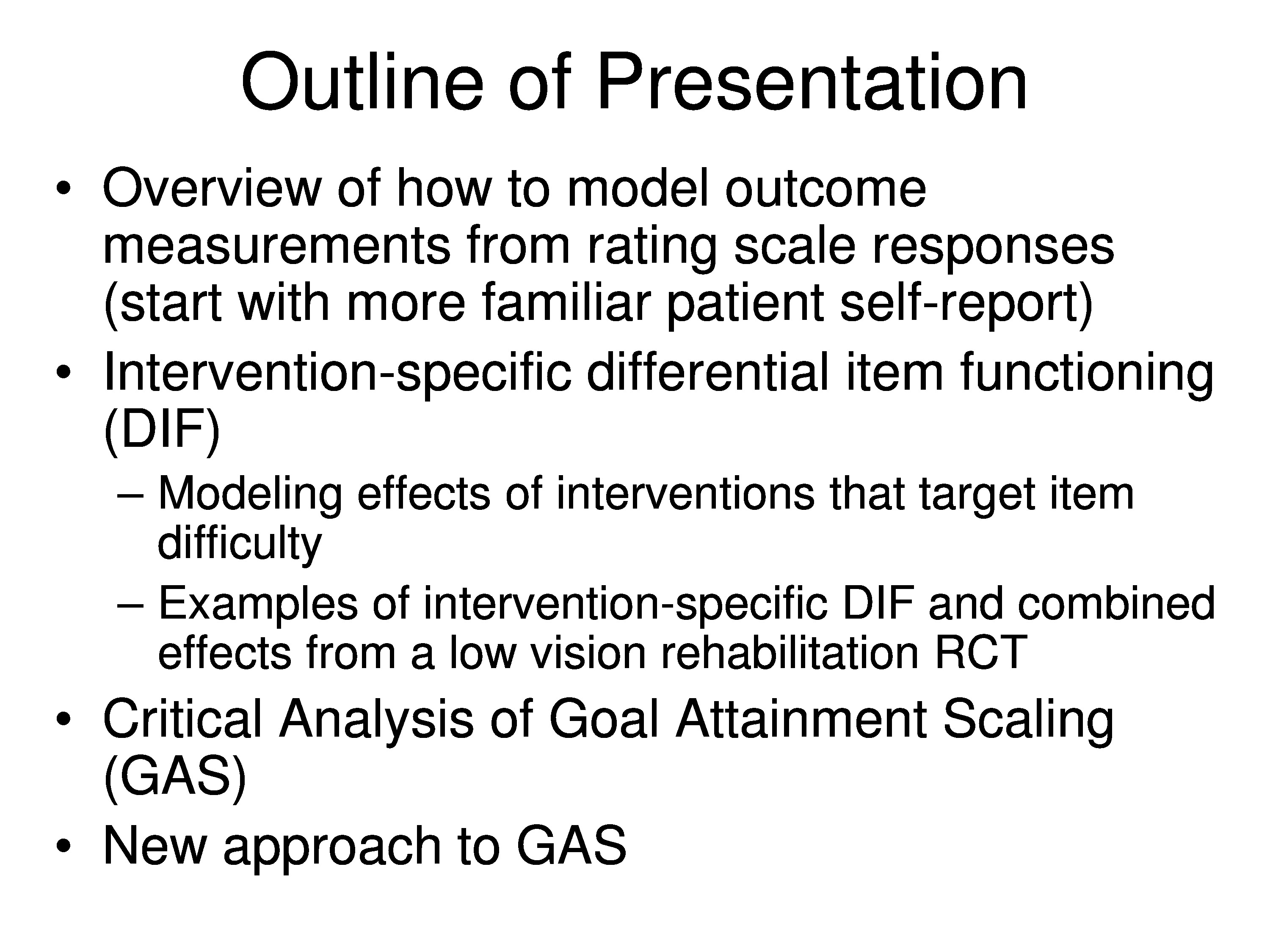
So what I’m going to tell you about, first, is kind of an overview of how to model outcome measurements from rating scale responses. And remember, this is a theoretical approach not a specific model. The specific model comes later.
To make it a little easier, rather than using GAS, we’ll start with patient self-report, the kind of questions we’ve been talking about through the meeting. I then want to get into the question of intervention-specific differential item functioning. And we’re going to be modeling the effects of interventions that target item difficulty. In other words, if you’re treating symptoms that you may change some of the items and have no effect on other items. And I’ll give some examples of intervention-specific DIF from my field in low-vision rehabilitation. And then we’ll finish with a critical analysis of goal attainment scaling and show a new approach to how we might implement this GAS strategy.
Measuring Functional Ability

Just to remind you, here is an overview of a functional ability questionnaire. In my field visual function measures, one of the instruments that’s popular is the VF-14, there are simply 14 items that describe everyday activities. The patient assigns a rating of no difficulty up through unable to do, and then has the option of saying not applicable, which is treated as missing data.
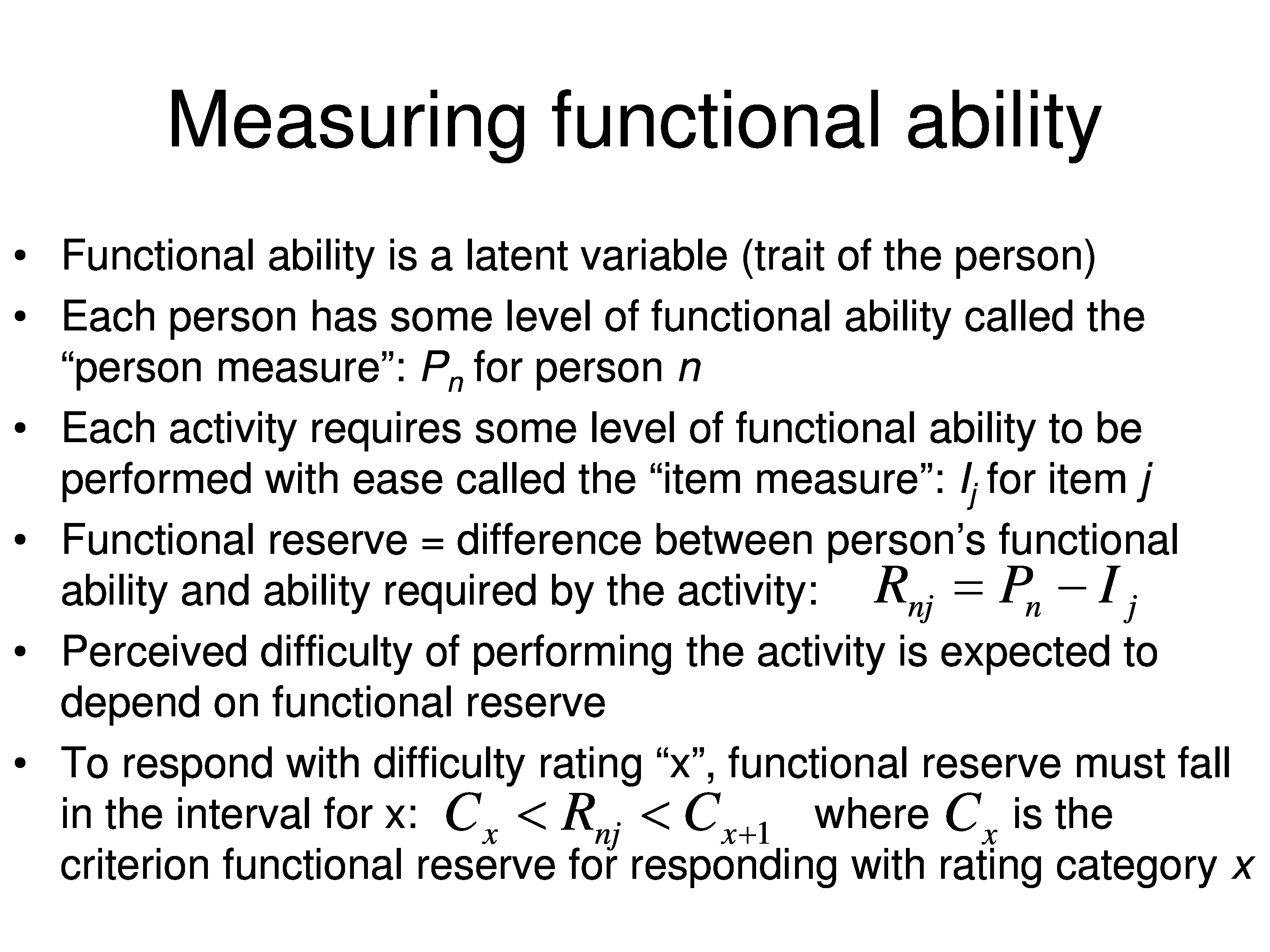
Functional ability is a latent variable and it’s a trait of the person. So you can substitute your own latent variable in for this. I’m going to use functional ability just so we have something substantive to talk about, but use whatever term you like for this latent variable. I’ll introduce the terminology I’m going to use. Each person has some level of this functional ability and we’re going to use a generic term person measure, so when we refer to that we’ll use a symbol P to represent person measure and subscript n for a specific person n: Pn
Each activity requires some level of functional ability to be performed with ease, and we’ll call that the item measure. And I will use the symbol I for item measure, subscripted j for the index for the item: Ij.
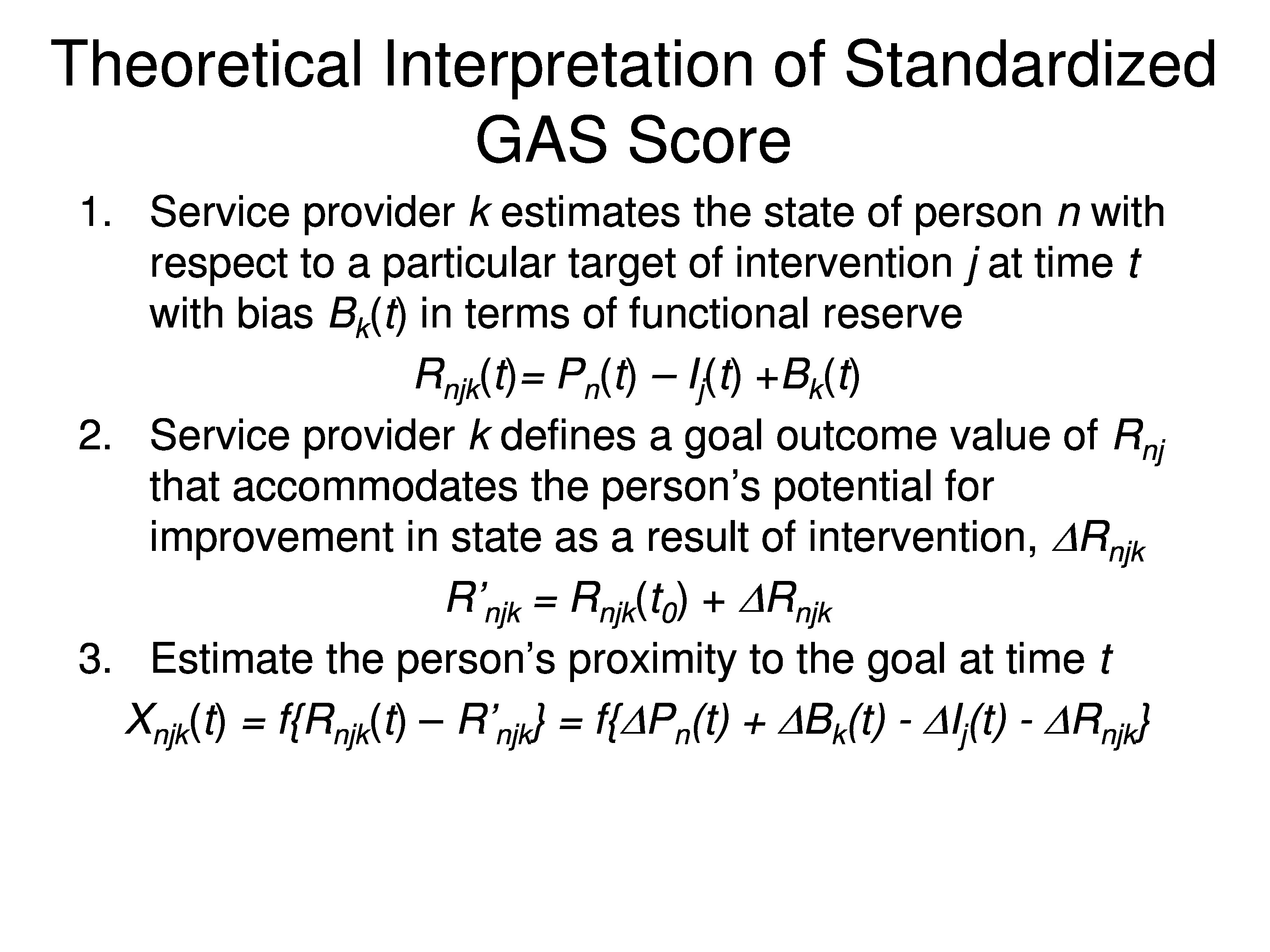
We’re going to introduce the concept of functional reserve, which is simply the difference between the person’s functional ability and the ability required by the activity.
So person-measure tells you how much you have, the item measure tells you how much you need in order to endorse the item. Functional reserve, or some other term if we’re not talking about function, is simply the difference between the person measure and the item measure. And I’m using the symbol R for a reserve and a subscript both for the person and for the item, which is just the difference between P and I: Rnj = Pn − Ij.
Now, what we’re asking the person to do is judge the difficulty of performing an activity. And our expectation is that their perception of the difficulty performing the activity, is going to depend on the functional reserve. So in other words, if the person has far more ability than is required to perform the activity, they should tell you it’s easy to do. On the other hand, if the amount of ability that they have is less than what is required to do, there’s a high probability they’re going to tell you they can’t do it. So concerning those extremes and everything in between, as the amount of functional reserve changes, you would expect that the estimate of how much difficulty it’s going to take will vary with functional reserve.
To respond with a particular rating category, we’ll use x to indicate which ordinal rating category we’re responding with. Functional reserve has to fall into an interval that’s defined by the patient. So the criterion or the category threshold, which is symbolized by C: the functional reserve has to be greater than the category threshold to respond with category x, but it has to be less than the category threshold to respond with that category x + 1. So C, then, is just a criterion that is set for that response category.
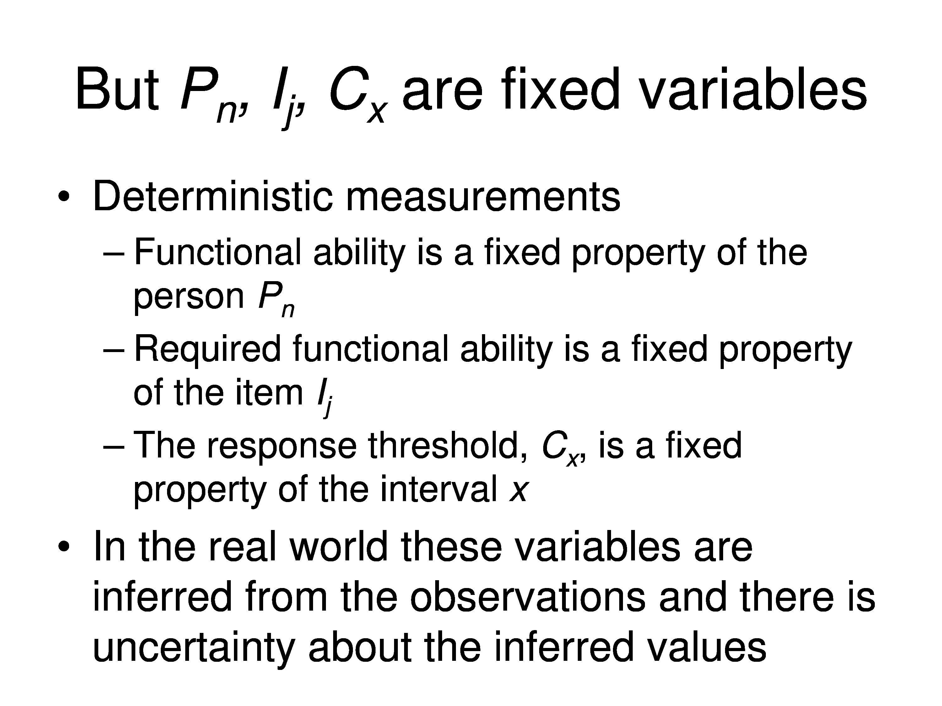
But the problem here is that P, I and C, the person measure item, measure, and category and threshold, are all fixed variables. It’s a completely deterministic measurement.
We can probably agree the functional ability is a fixed property of the person, but what we’re saying here is the required functional ability is a fixed property of the item, which may not true. And that the response threshold C is a fixed property of the interval, which most certainly is not true. In the real world these variables are inferred from the observations and there is uncertainty about the inferred values.
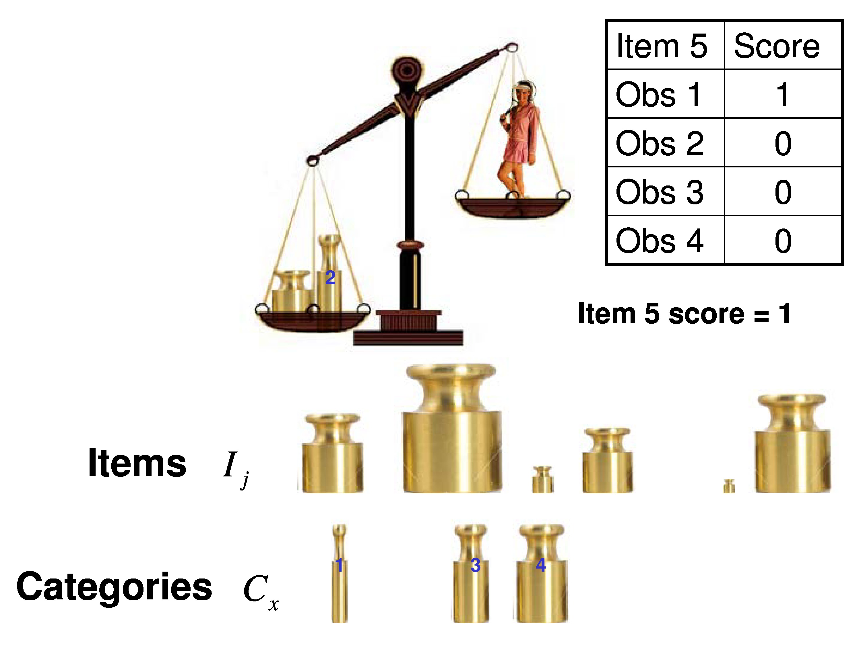
If you have a measurement theory or measurement model that’s worth its salt, it ought to be able to explain its physical measurements. So we use, as a metaphor, a balance scale.
So the trait of the person, in this case weight – but it can be any other trait functional ability — is being compared to the trait of the item, which is the same thing. In this case, weight, but it would be something else, and we’re simply dichotomously scoring each comparison.
We’re going to compare the person to every item and we’ll score it a 1 if the person’s heavier than the item. We’re score it a 0 if the item is heavier than the person. That would be a dichotomous scoring system.
If we want to do a polytomous scoring system we need another set of weights. In this case well call the categories. So for each item you would put the, for example, category 1 weight in with the item and we find that the person’s heavier than that combination of the item plus the category, so we’d give it a 1. We put category 2 in, in this case in this example, the item weight plus the category are heavier than the person, so we give it a zero.
Because we know those category weights are rank ordered by weight, all the rest of them have to be zero since they’re heavier than the one that got us here. So we give them all a zero. We add up those dichotomous scores. In this case we get a 1, but that’s the polytomous score would be the response for each of those categories.
Assumptions of Measurement Theory
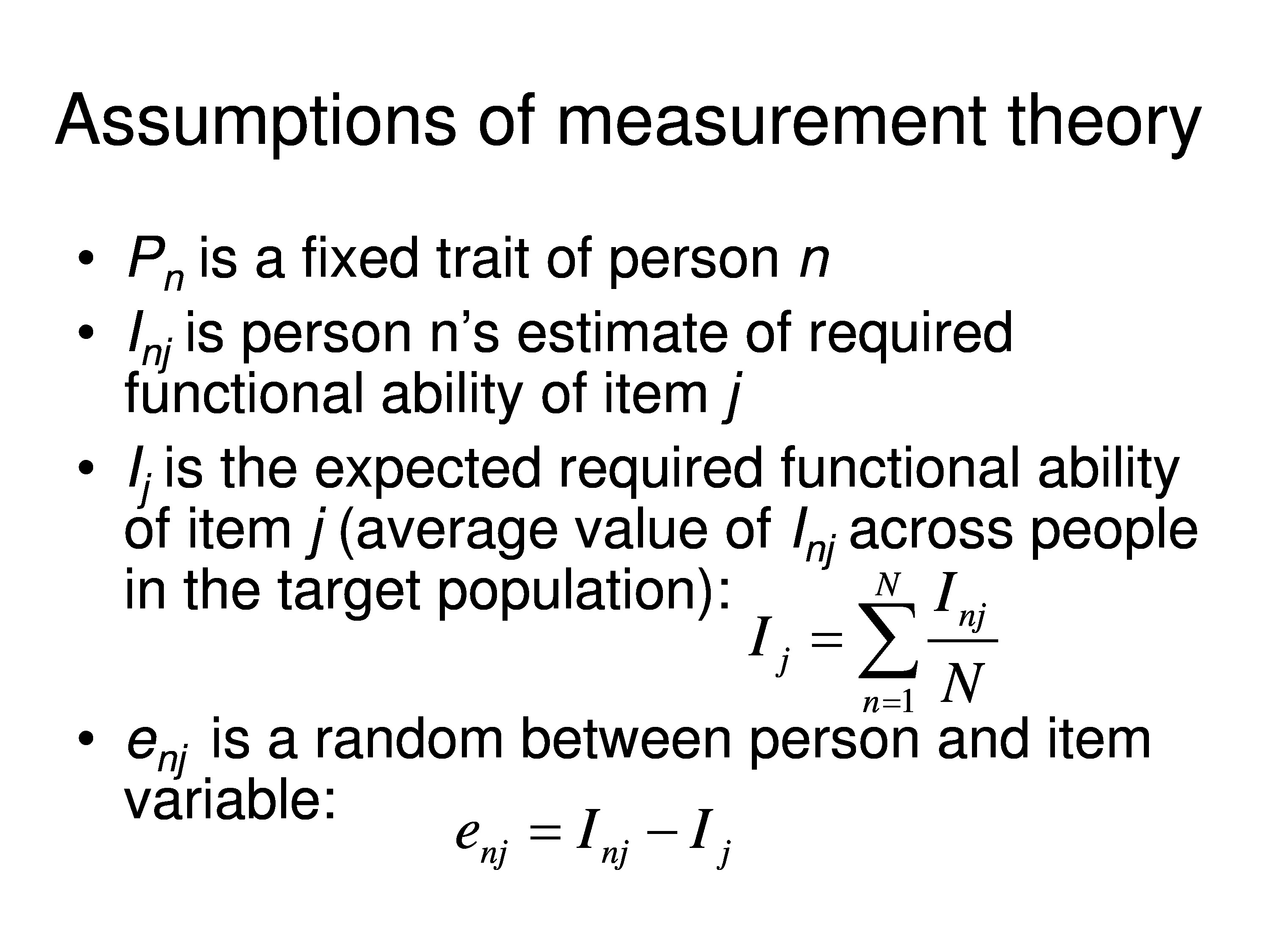
So for measurement theory, the kind we’re using, Pn is a fixed trait of the person, but each person is going to interpret the item. So in my field if we ask how difficult is it to read, one person’s thinking, well, I’m sitting at home with my 100 watt bulb in lamp reading the USA Today, the other person we ask that same question about reading a newspaper they might say, I’m sitting at home with my 40 watt bulb in my lamp trying to read the Wall Street Journal or the New York Times. And it might be different tasks, but the question isn’t specific enough so it allows for individual variations in the interpretation of I. So the item measure is really going to be indexed to the person in addition to being indexed to the item.
The fixed variable, Ij, can be interpreted as the average I, across your population, that you’re interested in studying. So my case would be the population of visually impaired patients, your case would be a different population. The average value of that variable is the fixed variable that we’re trying to estimate.
We then can define a random variable, which we’ll just use Ee for error, and that random variable is the difference between the I for the person and the average I for the population — and we expect this to vary both across people, randomly, and across items.
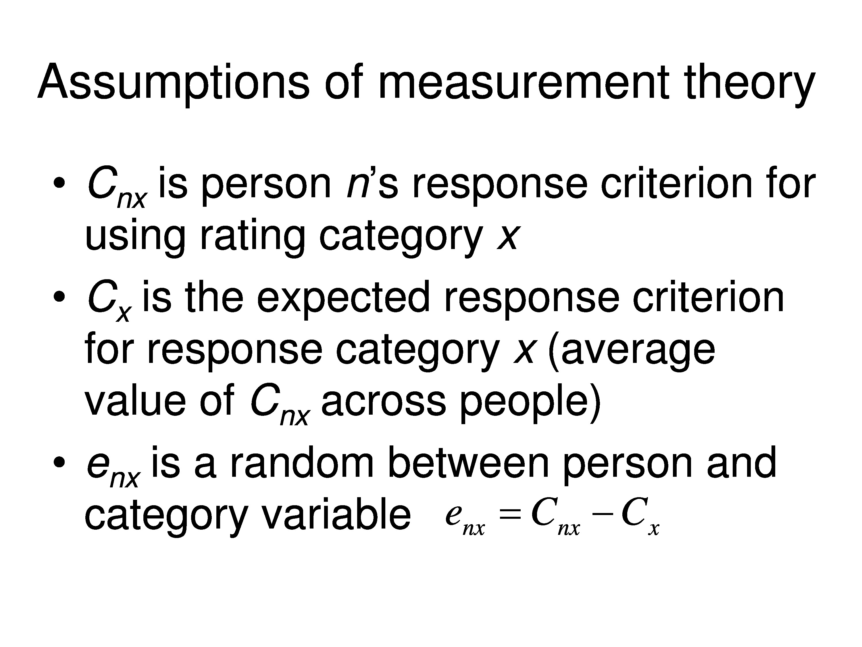
Similarly, each person creates their own categories. And so the category thresholds would be subscripted for the person. So the category for threshold for x would be Cnx, and that’s person n’s response criterion for using rating category x. And Cx, which is a fixed variable, would be the expected response criterion for response category x for your population. In other words, it’s the average value of Cnx across all people.
And then we would have an error term associated with that. Again, we’ll use e, but we’ll subscript it nx, and that’s just the difference between the person’s category threshold for category x and the average for the population.
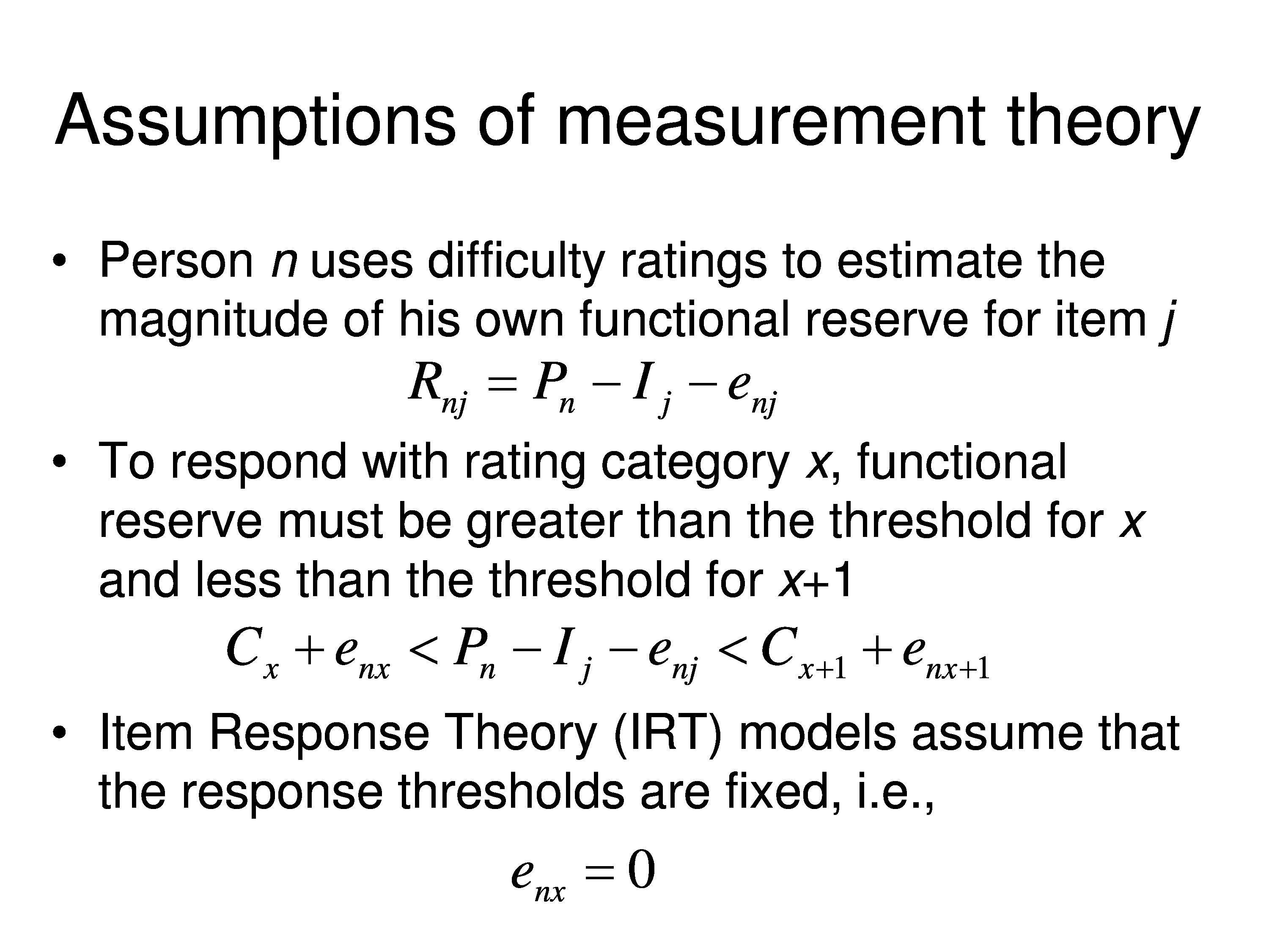
Now, person n is using difficulty ratings to estimate the magnitude of their own functional reserve for a given item. And so in this case now, functional reserve would be the difference between the person measure fixed variable, the average item measure fixed variable, and the error term that goes there.
So to respond with rating category x, functional reserve has to be greater than the threshold for x, and less than the threshold for x + 1. So now we put in the fixed category thresholds, which are the average for population, Cx and Cx+1. And there are errors associated with those category thresholds, and then we still have the error for the fixed variables on person measure minus the item measure. So this describes the conditions that have to be satisfied in order for the person to use response category x given the assumptions we’ve made up to this point.
Just as a side note, the rated response model that a lot of people use in item response theory, assumes that the error term on C, enx is zero for all values of n and all values of x. They don’t make that assumption explicitly, you just have to assume that in order to derive the graded response model.
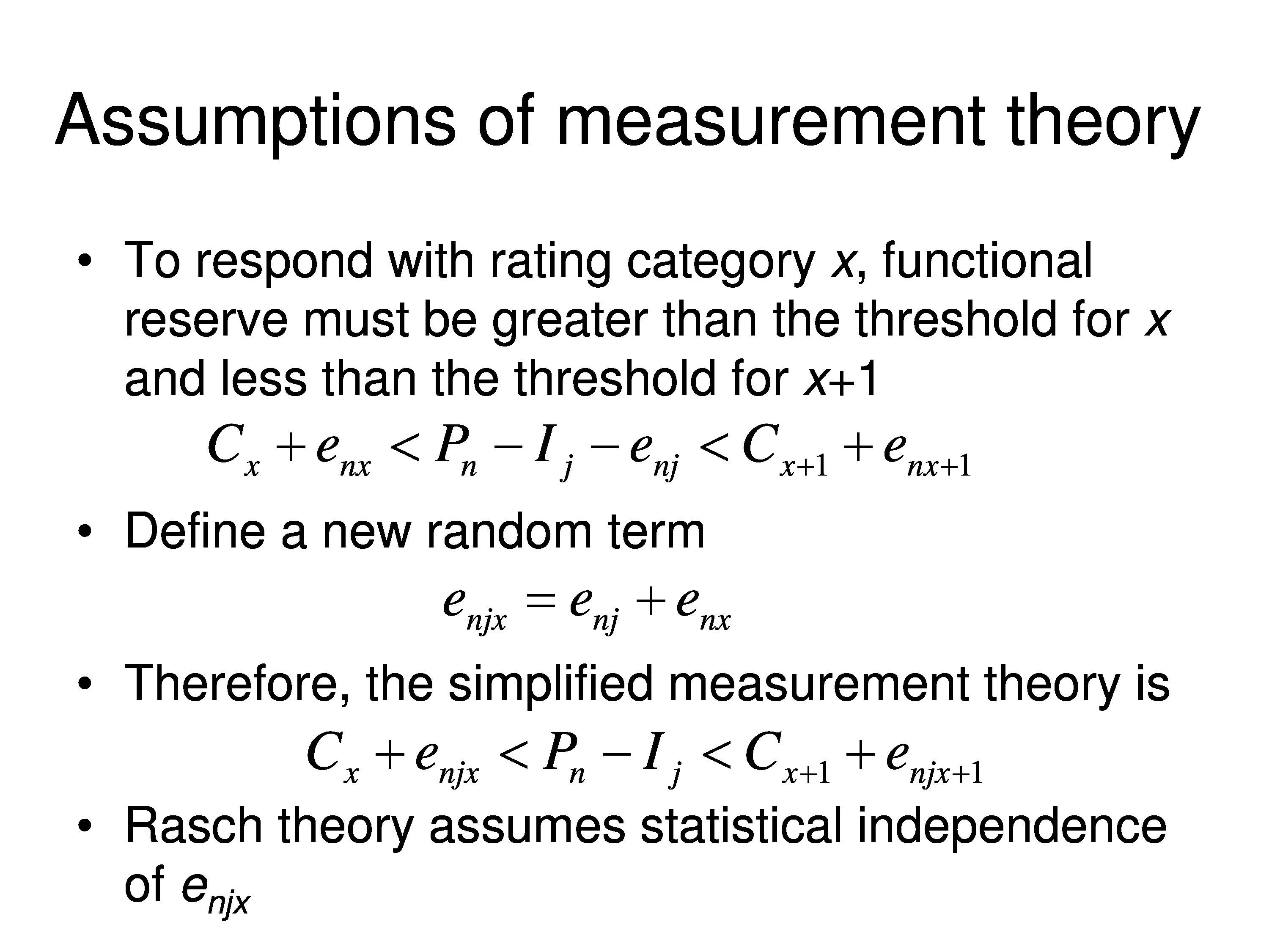
Okay, back to the story. To respond with rating category x, functional reserve has to be greater than one threshold less than the other threshold. So what we can do here is define a new random term. What we’re going to do is take enj and add it to every term. And so we’ll create a new random variable called enjx, which is just the sum of the two random variables we’ve defined. And now we can write the measurement, the scaling theory, just in terms of the two fixed variables Pn and Ij where Ij is the average. And the average category thresholds for the population, Cx and Cx+1, and then a random variable for each of those.
So that’s the theory. All the Rasch, IRT, confirmatory factor analysis, all the stuff you’re doing starts here. And every one of those things can be derived from this simple equation, simply by making specific assumptions about the distribution of the random errors.
And the models differ from one another based on the kinds of assumptions that are made about those distributions. Rasch Theory, in particular, all Rasch models, what they have in common is they assume that those random variables are independent of each other no matter what the indices are.
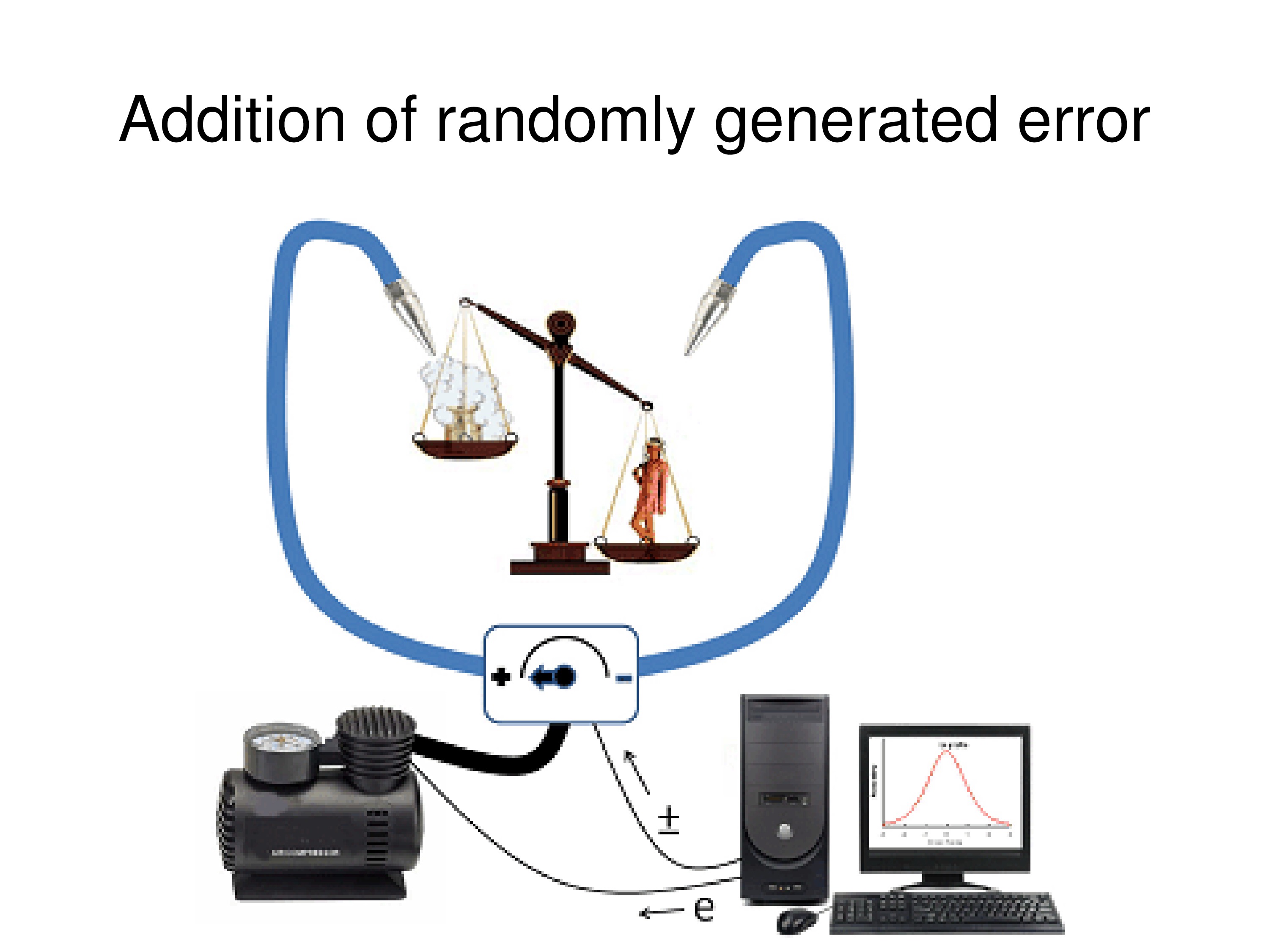
So how do we add that to our balance scale model? Well, we need a random error generator. So we’ll just put air puffs on the pans that are generated by a complex system that has a computer that controls how much force is going onto the platform and which of the two pans is getting the blast of air. And as you can see in the computer display it’s a normal distribution. We’re choosing from — on each trial we randomly draw a force from that distribution that’s average force is zero, and it’s either positive or negative, and then we blast one of the two pans that gives us our error.
If we blast the item pan it makes the item look like it’s heavier. If we blast the person pan it makes the item look like its lighter.
Example: Testing Validity

So, let’s go back to our VF-14 just to remind you of the real world. The task that we’re actually performing is asking the patient to rate the difficulty of performing each of these activities.
These are some actual data from the VF-14, and it’s taken from an Excel file.
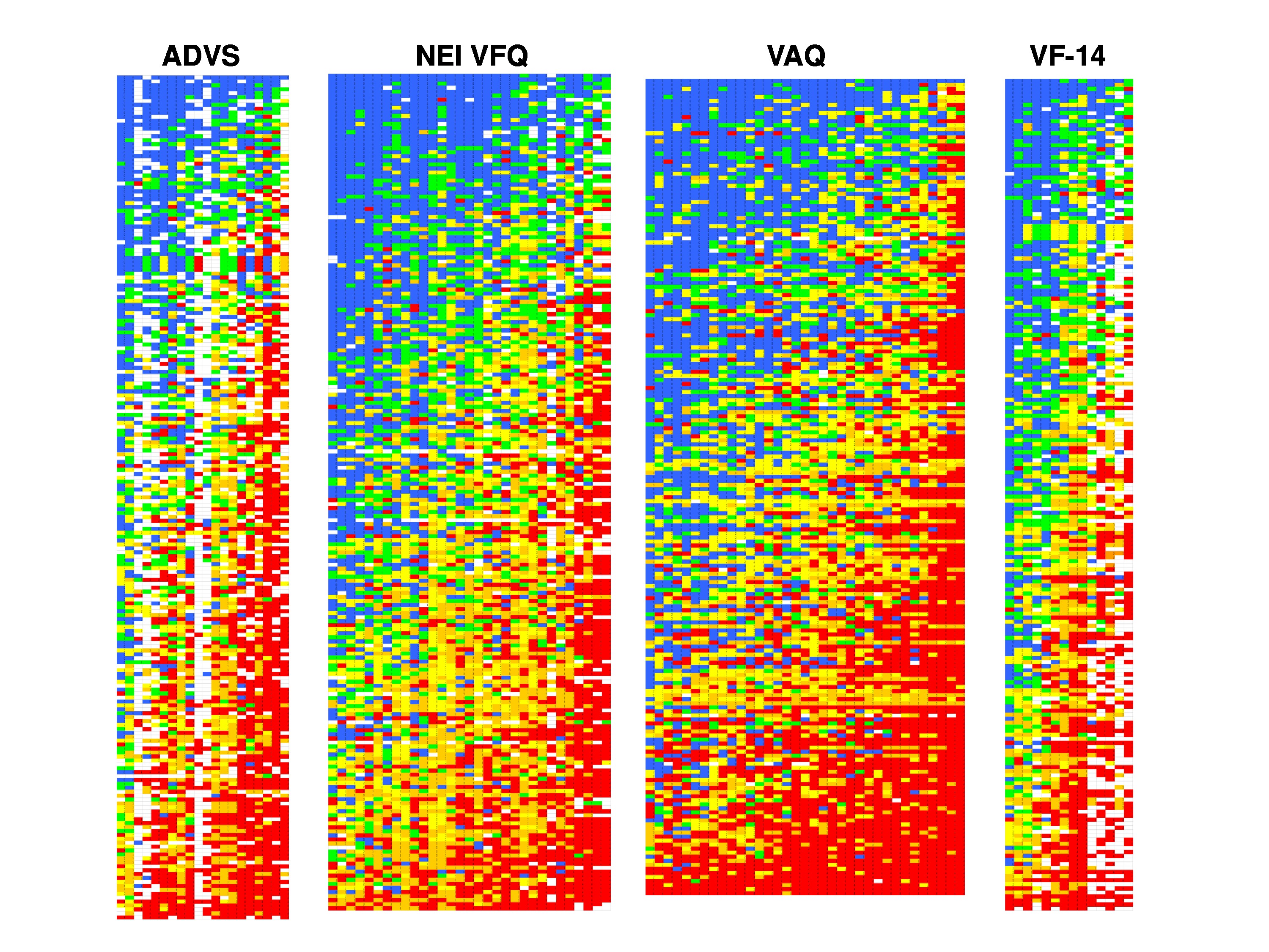
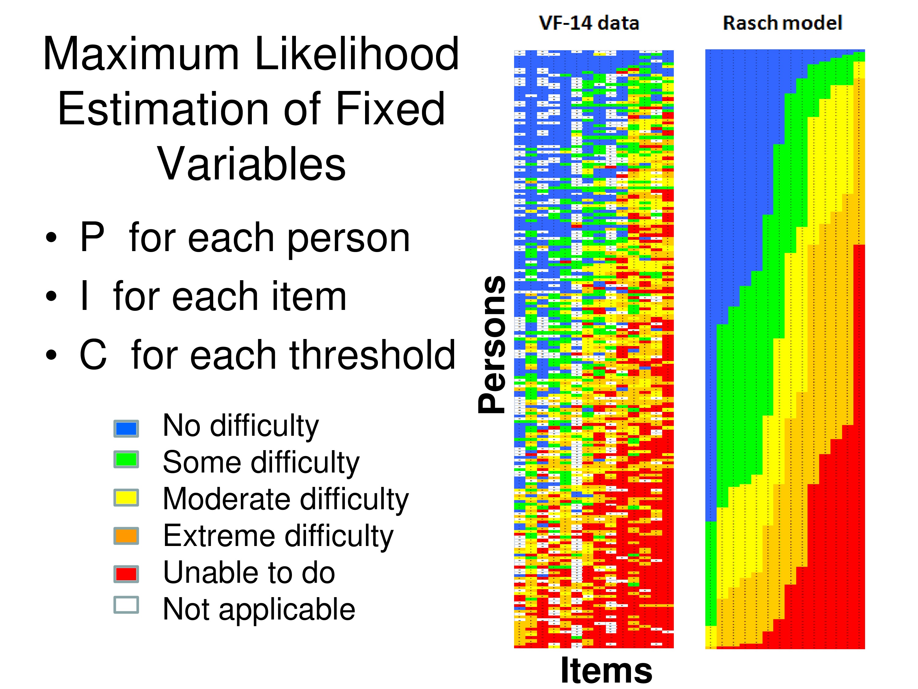
Look at the colored matrix on the left side first. Each column is one of the 14 items, each row is one of 200 patients, visually impaired patients who responded to the questionnaire, and the colors correspond to the response each person gave to that item. So if it’s blue they said it was no difficulty, up through red unable to do, and if it’s white that means it’s missing, they said it was not applicable.
You can see a banding pattern in the data, because what I’ve done is I’ve summed all the rank scores for the responses for each column across all the patients. And that’s the Rasch score for each item. And then I ordered the items by their Rasch scores. And then I summed across all items for each patient to get a patient Rasch score, and I ordered the patients by their Rasch scores.
So when we do that, if in fact we’re making a measurement, we should get what’s called a Guttman Scale. And a Guttman Scale would produce this banding pattern: that once you go from blue to green you don’t go back to blue again, you can only stay green or go to yellow. And then when you get to yellow, you can’t go back to green or blue you have to go to the next step or stay the same, to orange as you move across or move down.
What these measurement models do, once you make some assumption about the error, the measurement models then use maximum likelihood estimation techniques to estimate a person measure for each person, an item measure for each item, and a category threshold for each of these response categories in order to produce a Guttman Scale. The most likely Guttman Scale. And that’s what’s generated on the right side of that figure. The right matrix is the estimated responses by this group of patients to these 14 items based on the data themselves.

Now we can test validity. What are the accuracy of the assumptions that went into the model?
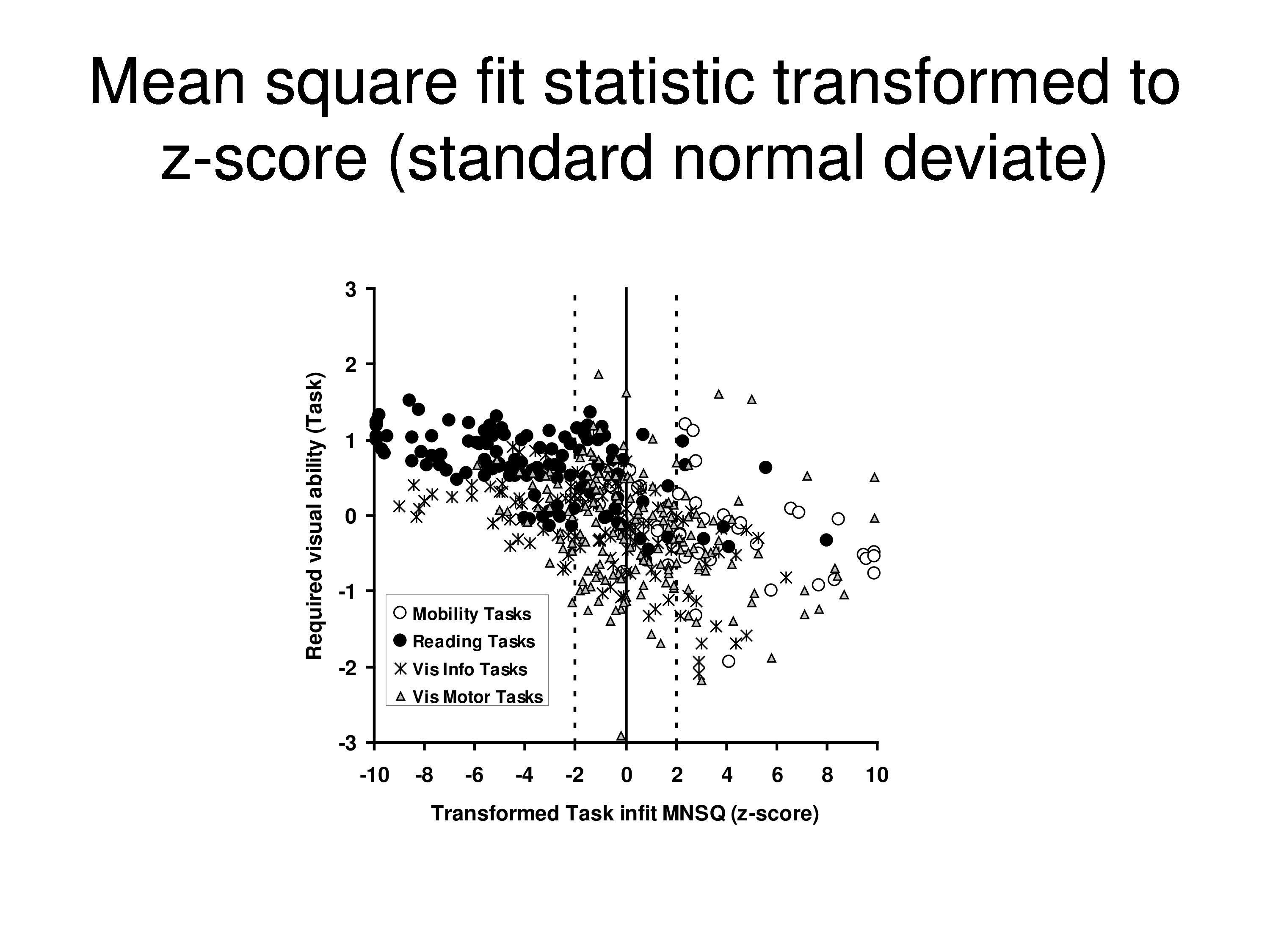
Well, we can do a mean square fit statistic for each person, and that tests the assumption that all the stochastic variance can be attributed to a single source in the case of a Rasch model. So there’s enjx is the error, that’s where the random variance comes from.
And we’ll take the mean square residual from each person. So we would take, we’ll start in the upper left corner and you take the response and subtract from it the expected response, which would be in the other matrix a corresponding sum of a neighboring matrix, and square it, and average over all items for that person. And that gives you a mean square residual for that person.
And you divide that, remember we have a model now that has a specific distribution built in. We divide that by the models predicted variance for each person. And that is called an information weighted mean square fit statistic or infit for short, and the equation below it is just putting in more attractive notation what it says in words above it.
And so, we have the actual observations, which are on the left. We have the expectations, which are on the right, which are generated by the model after we have done the maximum likelihood estimation. And we produce a ratio of the mean square difference, the mean square residual to the expected variance, to the predicted variance. And since we are using Gaussian distribution for the error, we expect these residuals to be distributed as chi square over its degrees of freedom. That’s just a property of this equation.
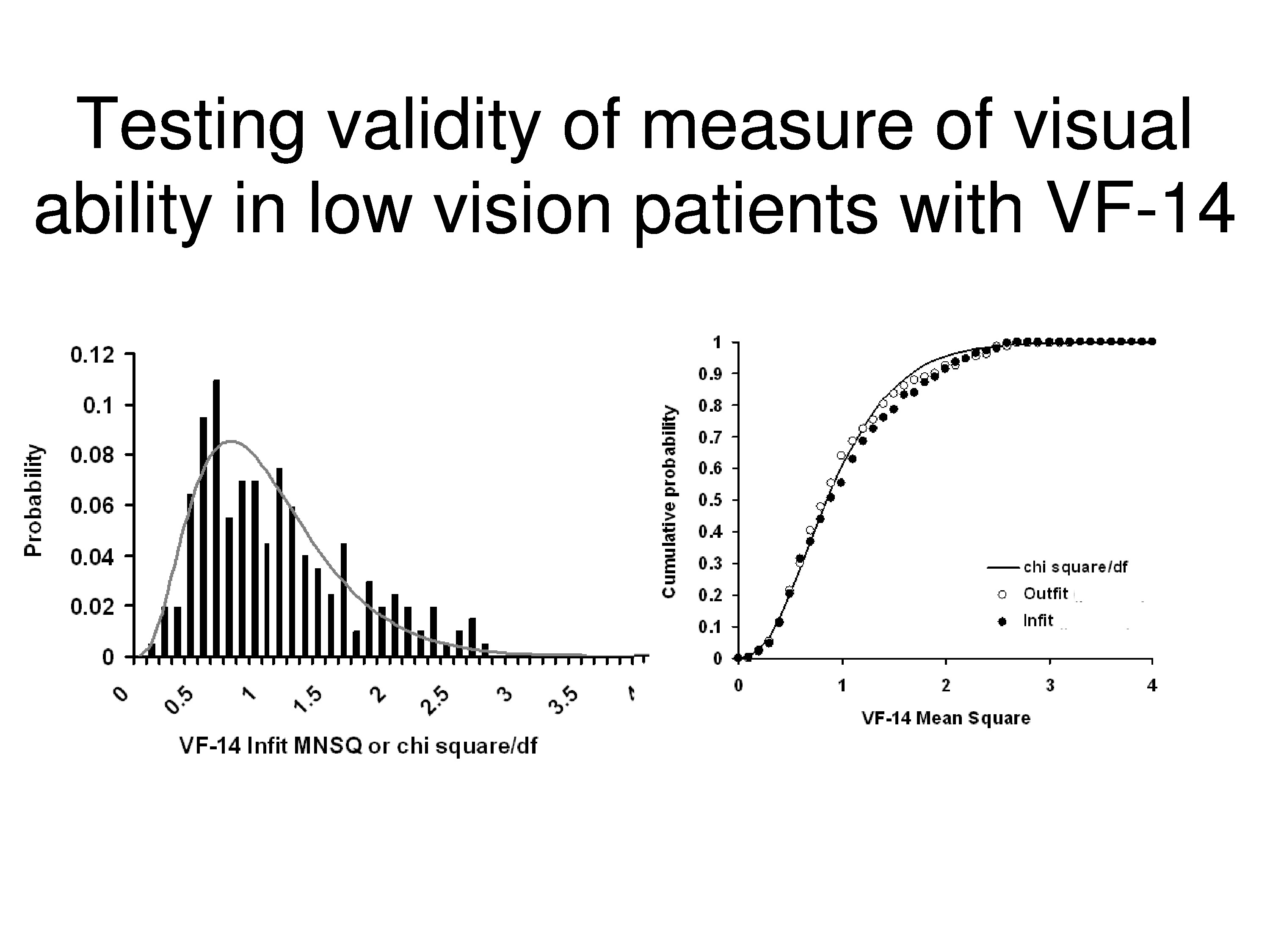
What’s showing on the left, the histogram, are the distributions of those information weighted mean squares, and the curve drawn through those data are the predicted chi squared distribution. The curves on the right are the same thing except those are cumulative distributions instead of the density functions, and I guess we could quibble over the little departure on the one part, but for the most part that’s a pretty good fit.
Just as a side note, this doesn’t necessarily mean you go start chopping off items because they are on the tail of the distribution. If the distribution fits than it’s meeting expectations of the model, it’s consistent with the expectations of the model. If you get outliers or you get faulty modes, or the distribution is just the wrong shape which often occurs, then that’s evidence you’ve got a problem.
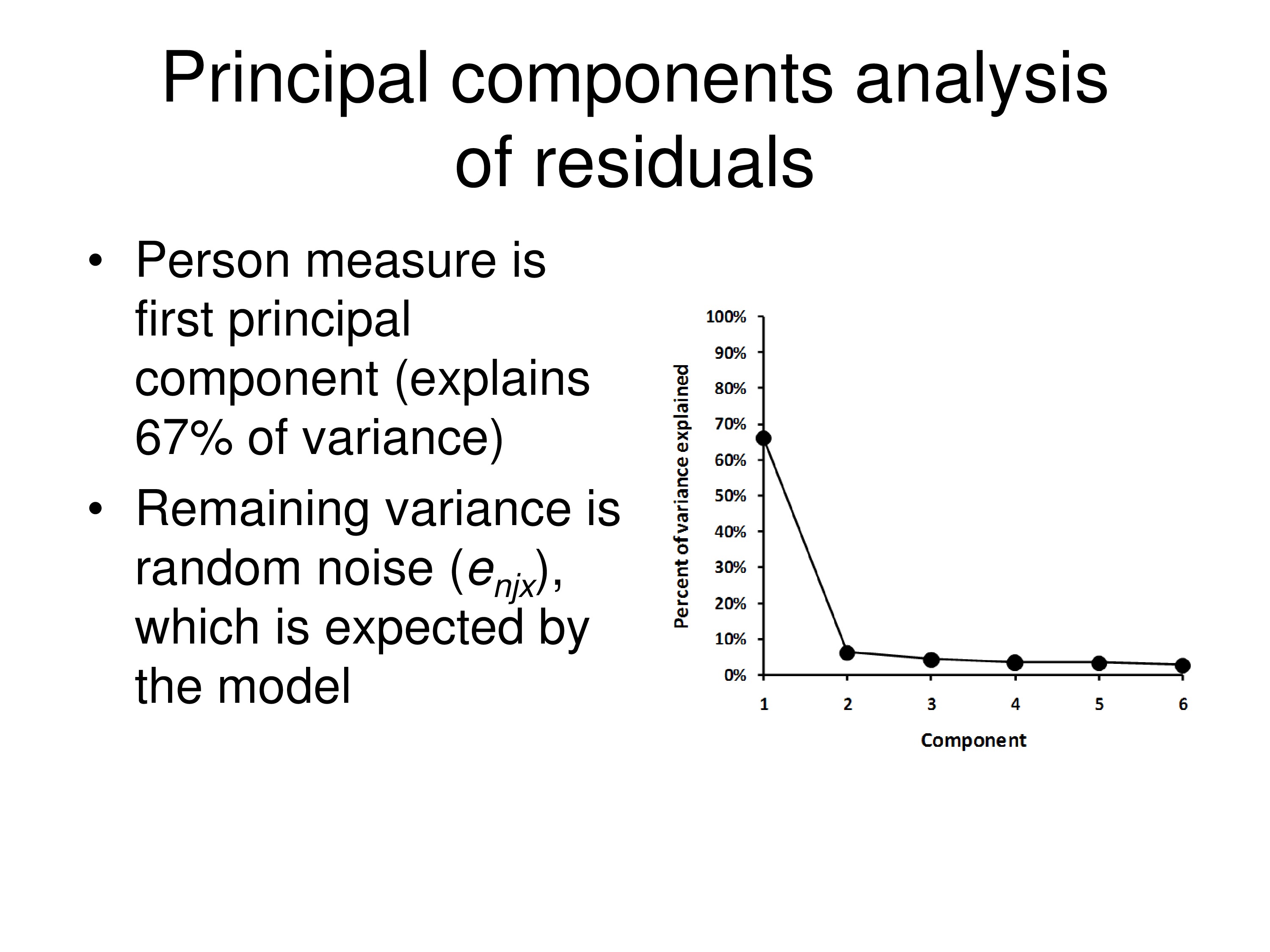
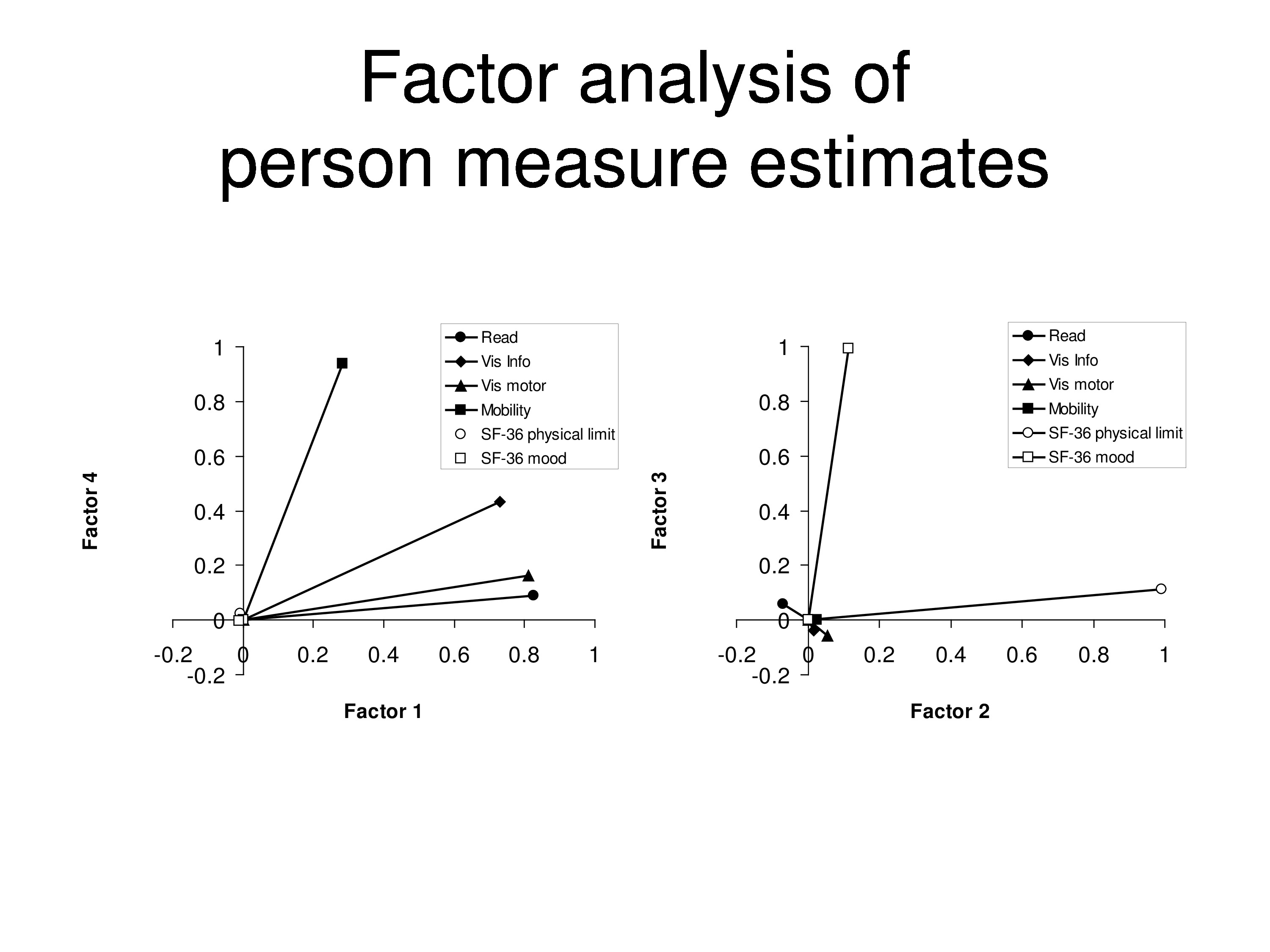
Go one step further — the assumption is all the variance should be the real variance in the distribution due to differences between people, and the rest of the variance should just be random noise. And so when we do a principal component analysis on the residuals we’ll find, first of all, the measure itself. The person measure explains about 67% of the variance in this data set, and then doing principal component analysis on the residuals we find the rest of it is just random errors.
So this particular instrument, the VF-14, given to a population of patient who have visual impairments, works very well. It’s a very good measure.
Effects of Intervention
Now, what about intervention? What’s actually happening?
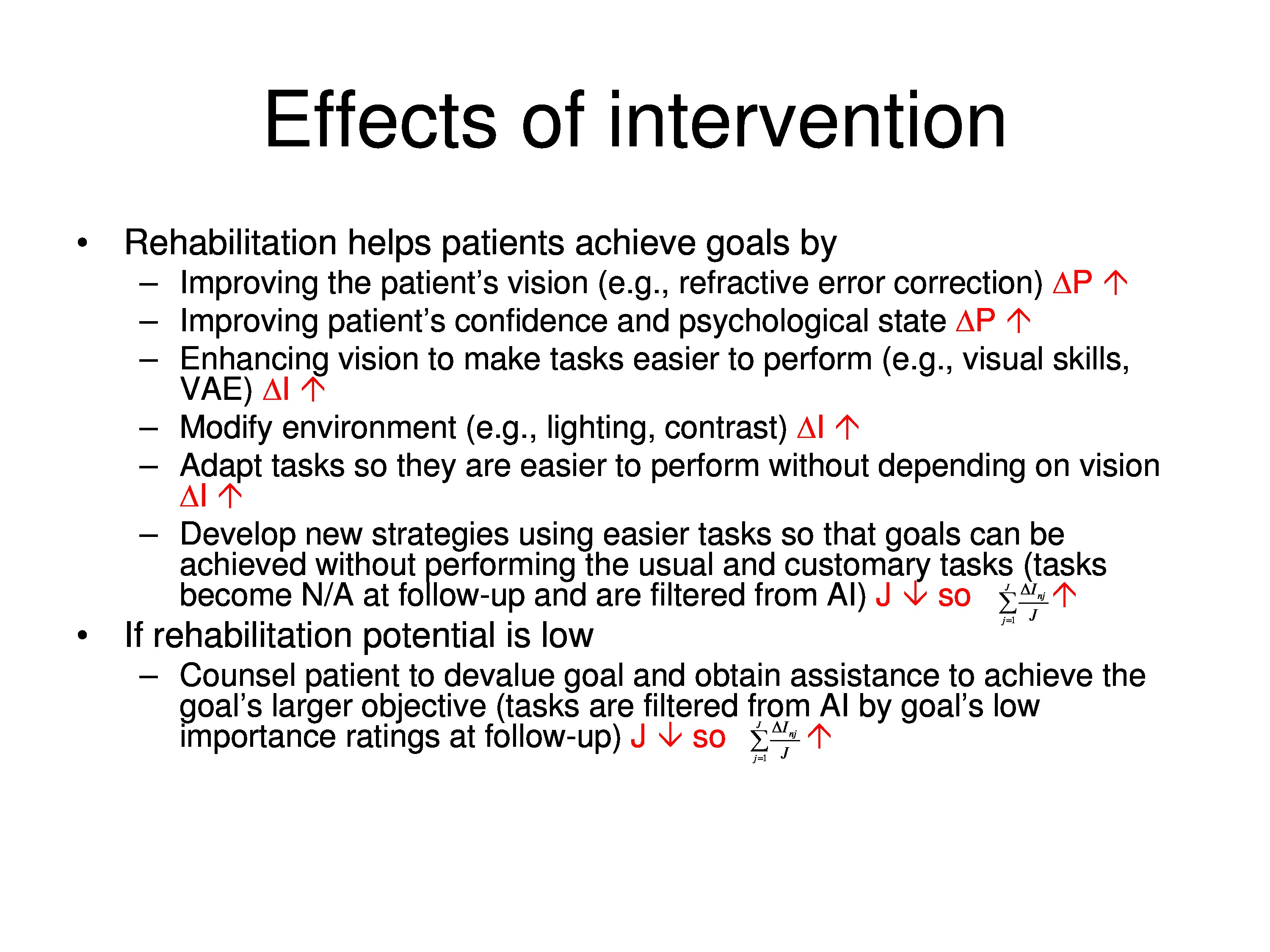
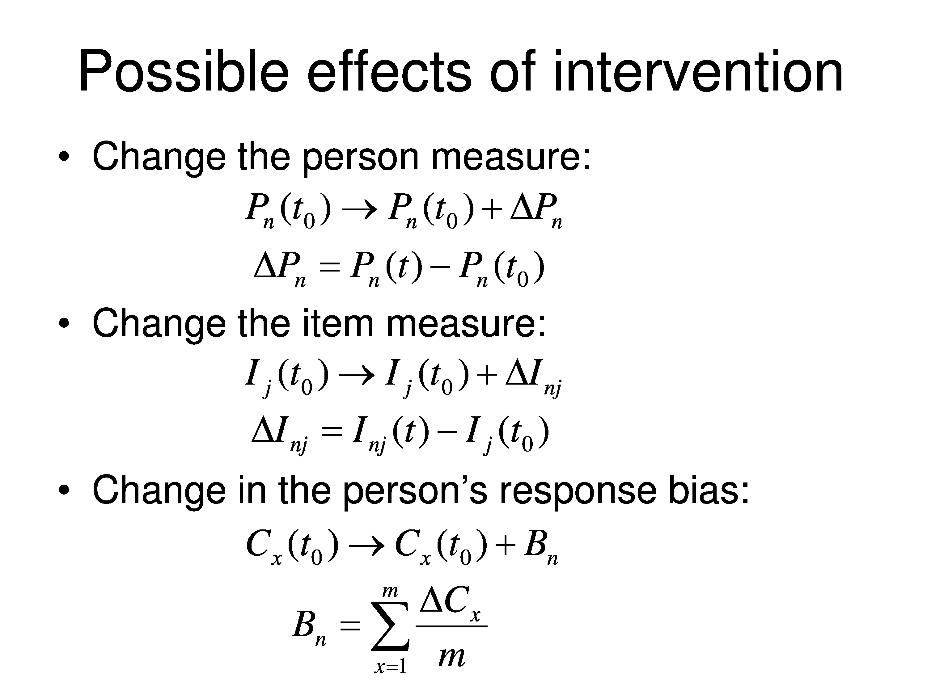
Well, one thing that could happen as a result of intervention is we can change the person measure. So the person measure at time t zero, which would be baseline, gets changed by some amount. Δ, the Greek letter, means change. So this is just change in the person measure. So it goes from the baseline value to the baseline value, plus or minus some change. Δ in this case is just the difference between the person measure at follow-up and the person measure at baseline.
We could also get a change in the item measure. The notation’s the same. We have an item measure for item j at time t0 baseline, and then we could change it up or down. So the change here is just the difference between those two.
Another thing that could happen is the patient is playing two roles. They are the object of the measurement, that’s what we want to measure, but they are also functioning as observers. They’re making judgments and reporting results.
In some cases, if the therapist is making the judgment the therapist is the observer, and so it is the same equation just different interpretation of parameters.
So in that case, the response criteria at baseline have built into them the person’s bias. We normally don’t express the bias separately, but the bias might change as a result of the intervention. The patient might be Hawthorne effect, the placebo effect, not necessarily real changes in the person or the item but just the way the person uses the response scale. And they’re more positive or overestimating their ability, something of that sort. So we represent bias with the letter B, subscripted for that particular person. And B can be thought of as the average change in all the category thresholds across all the categories.
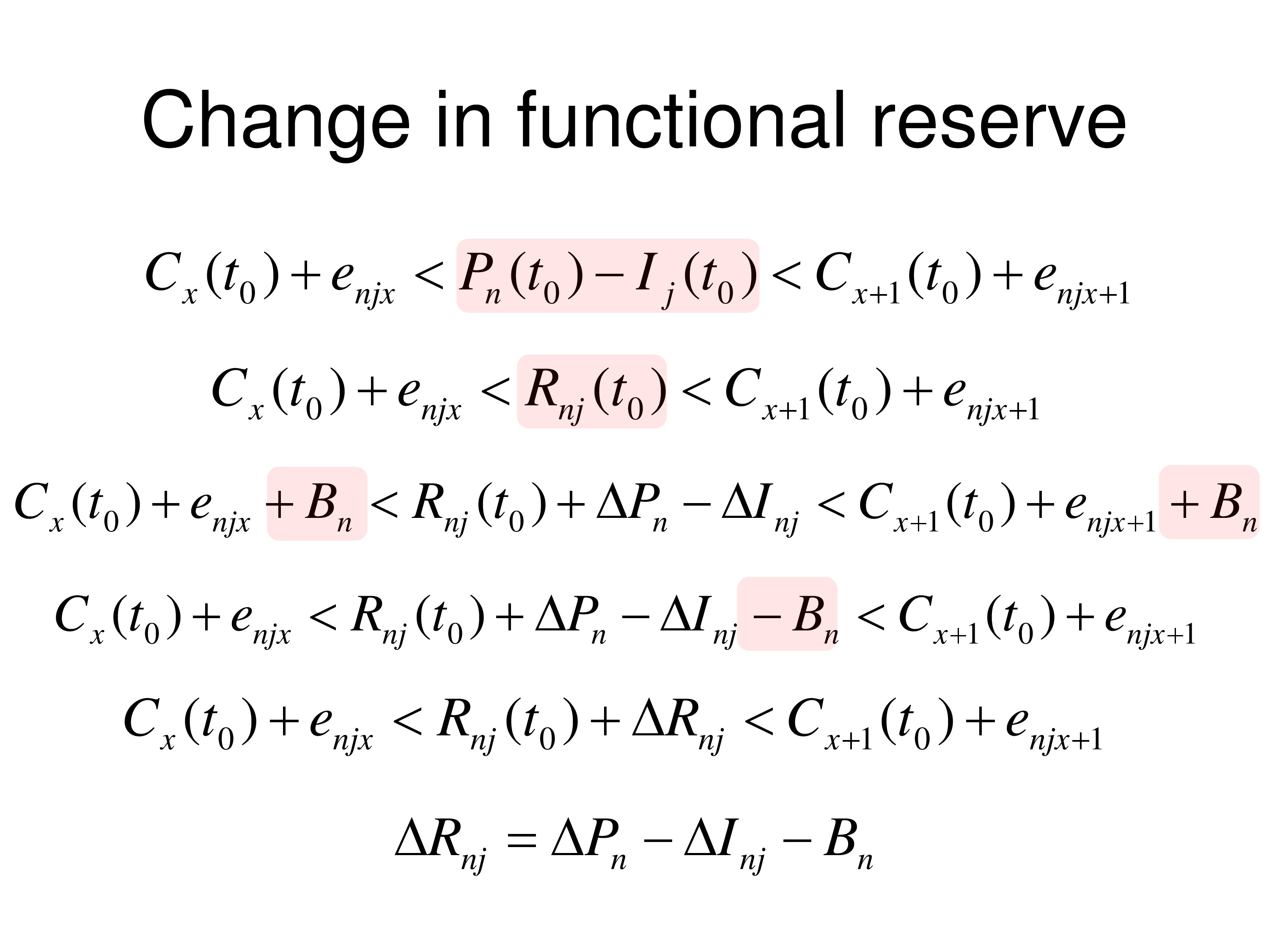
So now if we want to talk about the change in functional reserve the way we’d set up the theory is to, the way we did it before, we substituted the difference between people and just put the term functional reserve in, and we have other terms.
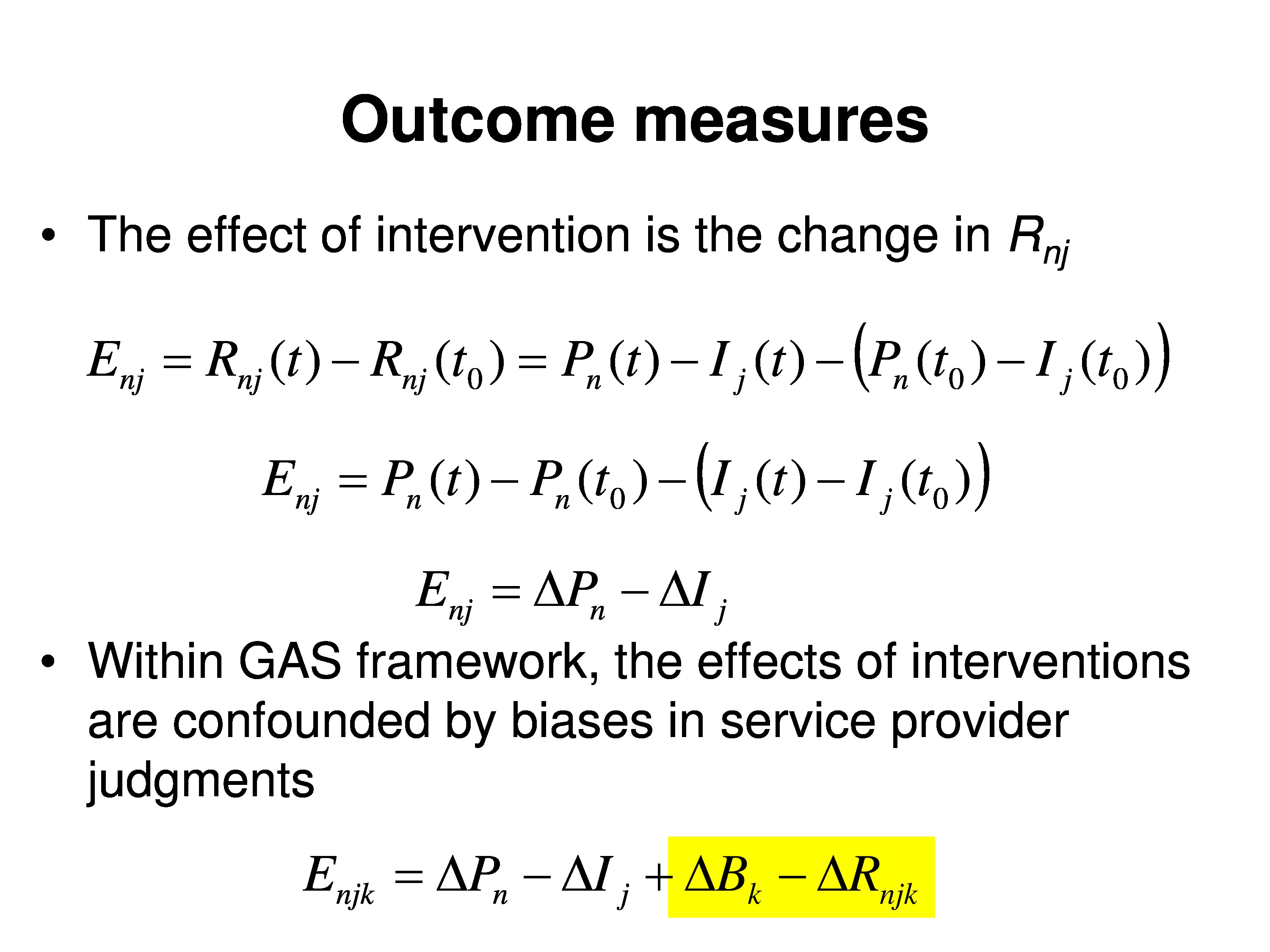
But now we’re going to add possible things that could change to this equation. B is the bias term, that could change. The ΔP, which could be a change of the person measure. ΔI could be changed in the item measure for that person, so we’re indexing it in.
And we can take the B out of this equation here and subtract B from everything and it will show up here so we can put all the terms that could be the outcome, we just add that to functional reserve.
And we could summarize those change scores, those change terms, with a single change in functional reserve ΔRnj, where that is just the combination of the terms that we collapsed into that.
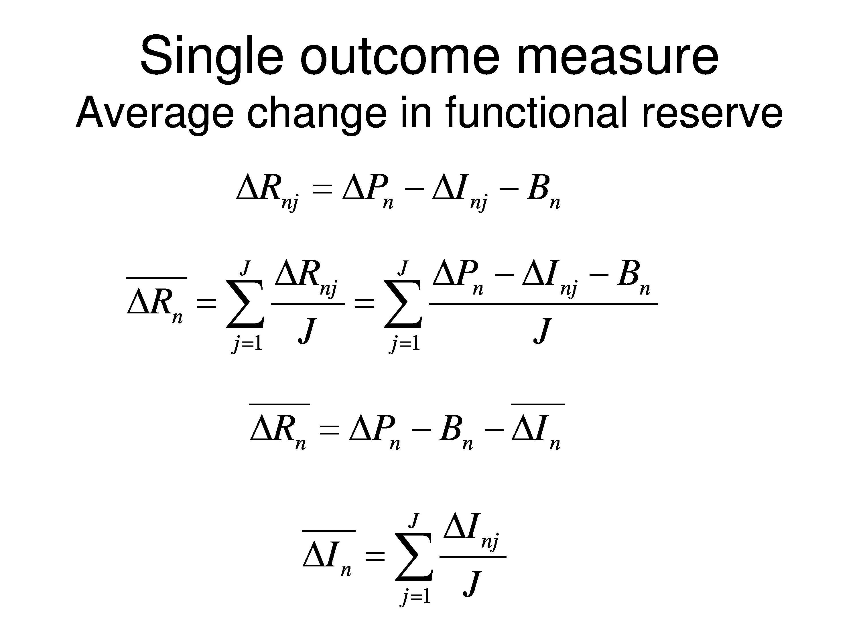
Just a repeat of that last step. Now what we want to look at is what is the average change in functional reserve. Because when we do outcome measures we want a single variable. We don’t want to have a vector of variables that we’re now saying treatment A is better than treatment B because these 20 variables changed more than these did. I mean, it would be a very difficult thing to sort out. So we want to talk about a single outcome measurement. So what we end up doing is averaging these changes across all the items for each person.
What you can see is, if you average the person measures across items, the change of person measures will stay the same. Average across items is the same as what it was. If you average the bias that doesn’t change across items. But if we average the item changes across items we get this ΔI event, which is the average of that specific to that person.
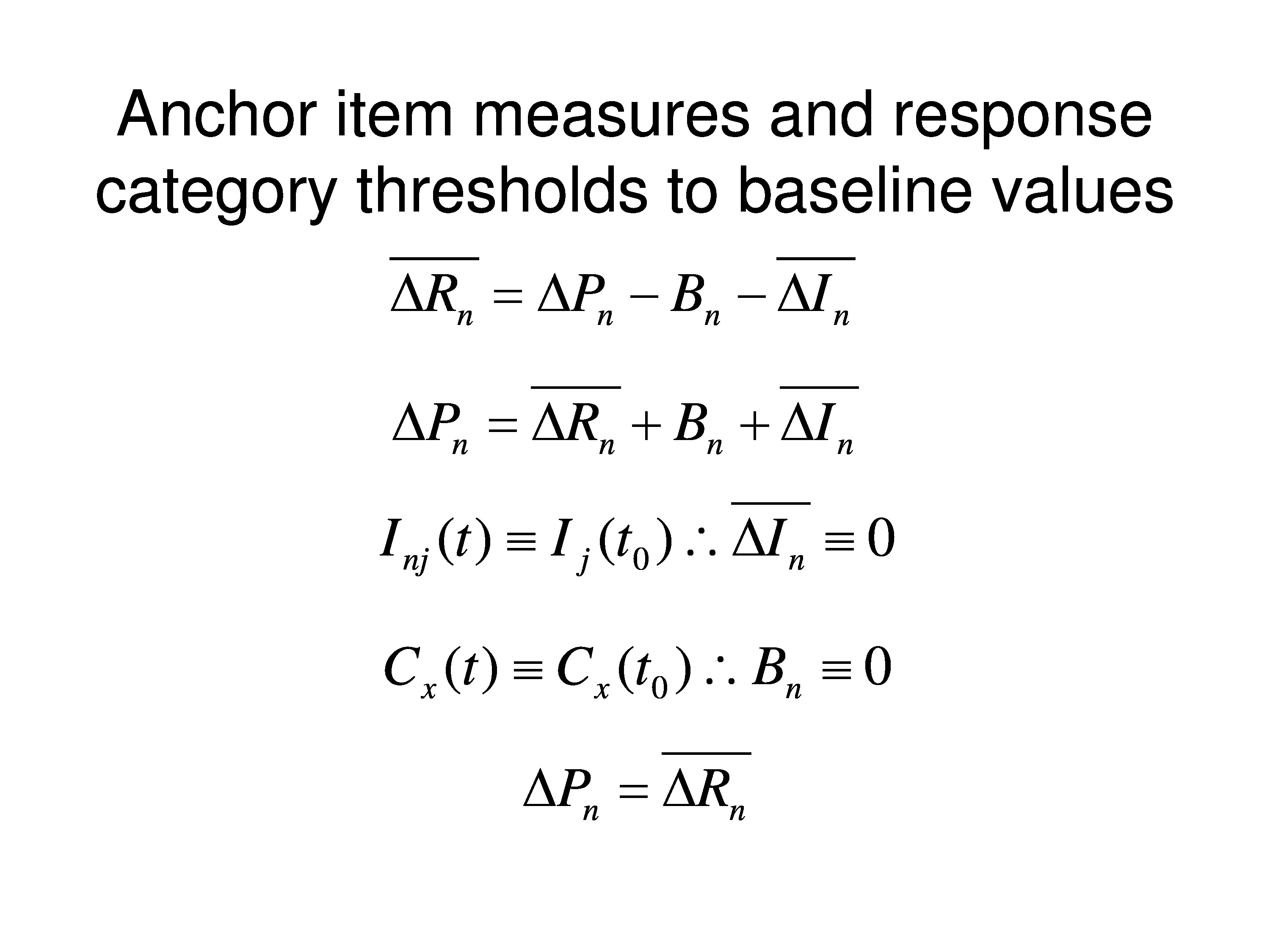
Now, what we would normally do is calibrate the instrument, you’ve heard a lot about that today, calibrating instruments and creating item banks and so on. So we’d anchor the item measures and we’d anchor the response category thresholds to their baseline values for the population that you want to study.
So what happens is that we can rewrite this equation for the average change in functional reserve to just a change in the person measure. Because if we’re anchoring the values, by definition there can be no change in the item. And by definition we’re not allowing singling out bias. So what happens is that all changes in functional reserve, which is what causes them to change their response to an item, we’re going to assign to the person measure. We’re going to say that it has been change of the person measure.
So like we just said, the item measure at time t is defined to be the same as the point of baseline, so that has to be zero. And the category threshold time t is defined to be the same as on the baseline so the bias change, the bias term has to be zero. So everything else — so all of those changes, if they are really occurring, we’re forcing them to show up on the person measure chains. And we’re defining the person measure change just as a change in functional reserve which is what is being judged when the patient gives their response.
Simulation
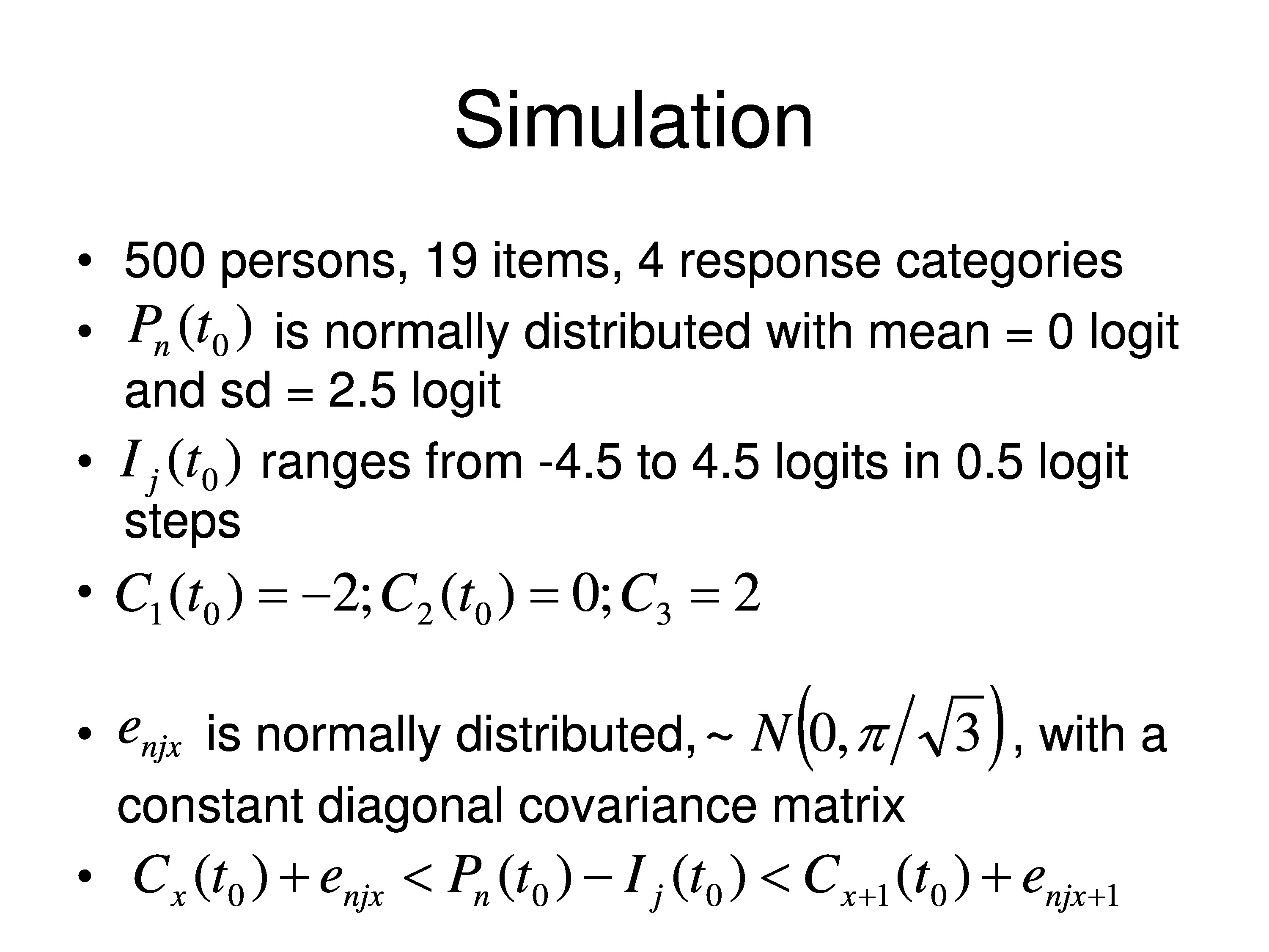
So to demonstrate this we’re going to do a simulation. So we’ll take 500 people, made up people that live in the computer. We have 19 items which also live in the computer. This is very generic, not even talking about what we’re talking about. And we’ll have four response categories.
We took the baseline person measure and say it’s normally distributed, it has a mean of zero logits and standard deviation of 2.5 logits. And the item measures range from minus 2.5 to 4.5, in equal steps .5 logits. And the category thresholds are minus 2 zero in 2 for the four categories.
Three category thresholds if you have four categories. First category is anything less than C1. Second category is between C1 and C2. Third category is between C2 and C3 Fourth category is anything greater than C3.
We assume that the errors are normally distributed around a mean of zero, and just a little technical thing, we make the standard deviation π over the square root of 3 because we’re using what’s called a logistic distribution. And that allows to normalize the distribution to be able to represent a normal distribution with a logistic.
And we assume there’s no correlations in this matrix of errors. In other words, enjx, it varies as function of person and it varies as a function of item, it varies across categories, and none of those things correlated with each other. They’re all independent. That’s what’s called local independence, which is what all these models use.
And then we have our magic equation at the bottom for baseline responses, and that’s how we generate the predictions. We grab a person, go right through all 500 people. We have a person measure for each one. We’ll start with a normal distribution. We’ll plug in the person measure, plug in the item measure, take the difference, take the category thresholds, add a random draw from this normal distribution from this category of errors and add them to the category thresholds, and then ask is it greater than 1, 2, 3, so on, and we define a response for that person judging that item in the computer.
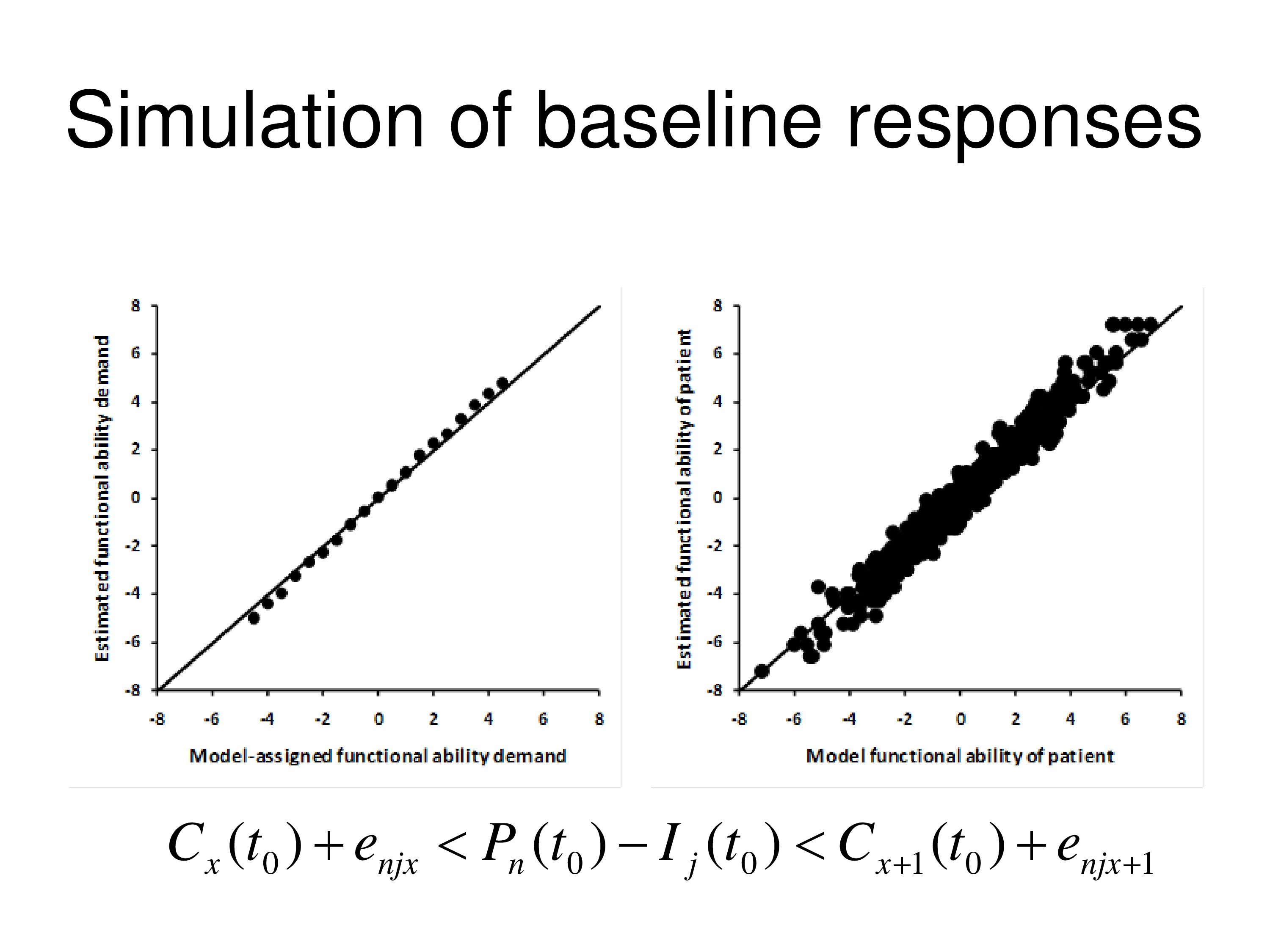
The graph on the left shows the item measures that are estimated by WINSTEPS, using a Rasch model, Andrich rating scale model, versus the items measures we’ve plugged into our computer to start with. You can see a pretty good agreement. And on the right is comparing the person measures for all 500 simulated people estimated by the WINSTEPS to the Andrich rating scale model versus the person measure we put in the computer. And the diagonal lines in both cases are the identity line, so it’s a line, slope 1, intercept of zero.
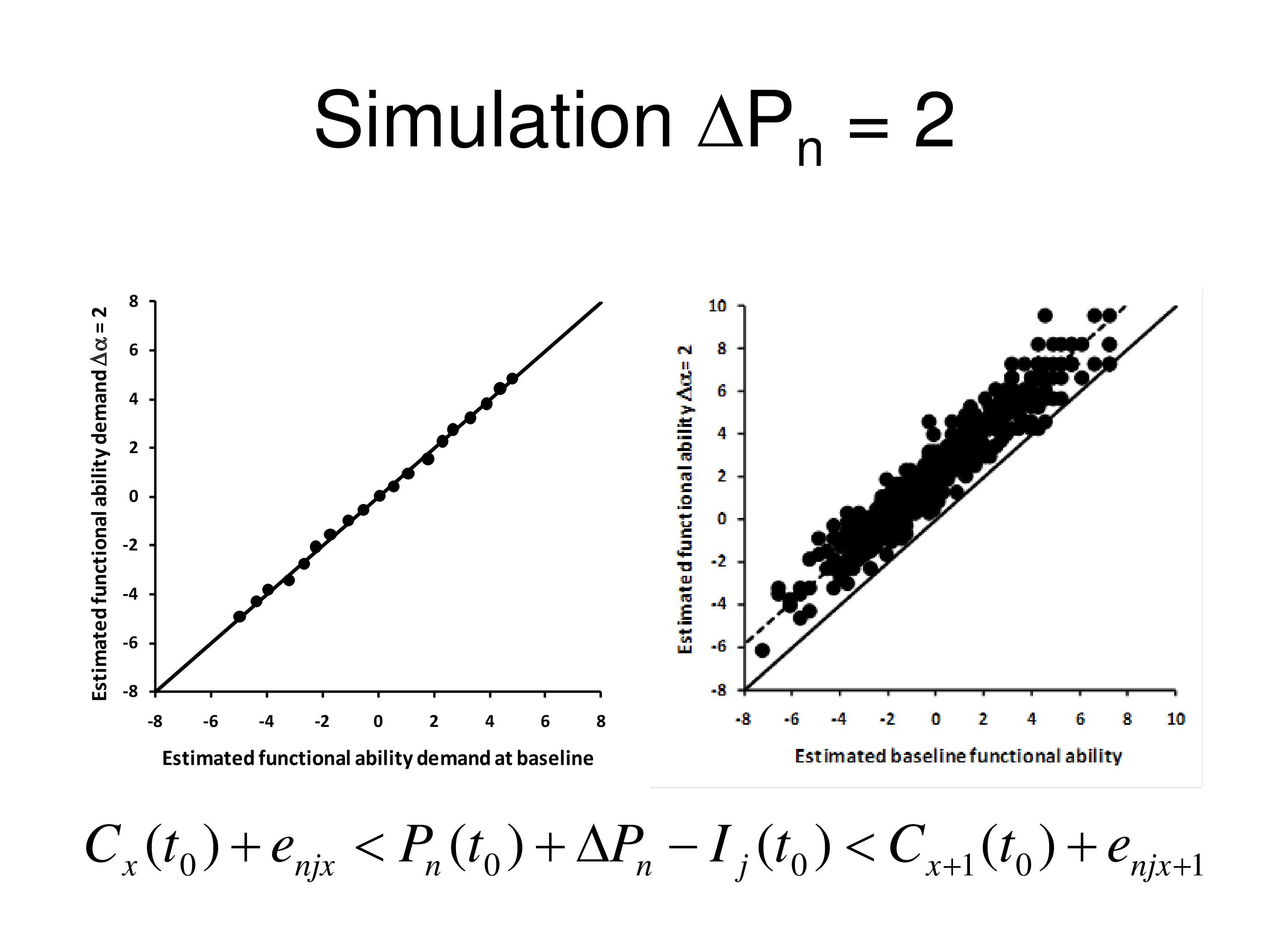
Now we put a ΔP in there. We say there’s going to be a change in the person measure by two logits, and we’ll say it will change everybody’s person measure by two logits. That is, the treatment has one effect, it changes by two logits. And so we put that in so we increase every person measure by two logits. We run it through the computer again, do it through WINSTEPS, and we compare the items measures. We’re not anchoring anything now. We compare the item measures we estimated from ΔP up by 2 to what we estimated at baseline, and the graph on the left shows the relationship between those two, perfect agreement between added measures. So incrementing ΔP didn’t do anything to the item measures. But person measures all went up by two logits. So they’re on a line that has a slope of 1 but an intercept of 2. It went up by two logits above the other one.

Okay, now let’s write the equation with the bias term and the category thresholds. And we’ll set the bias term as a change in two logits for everybody. And when we run that, same thing, on the left the items don’t change, but on the right, what we get is person measures fall down by two logits. So bias term acts the same way ΔP does. Change in person measure or change in bias can’t be discriminated, they act the same way.
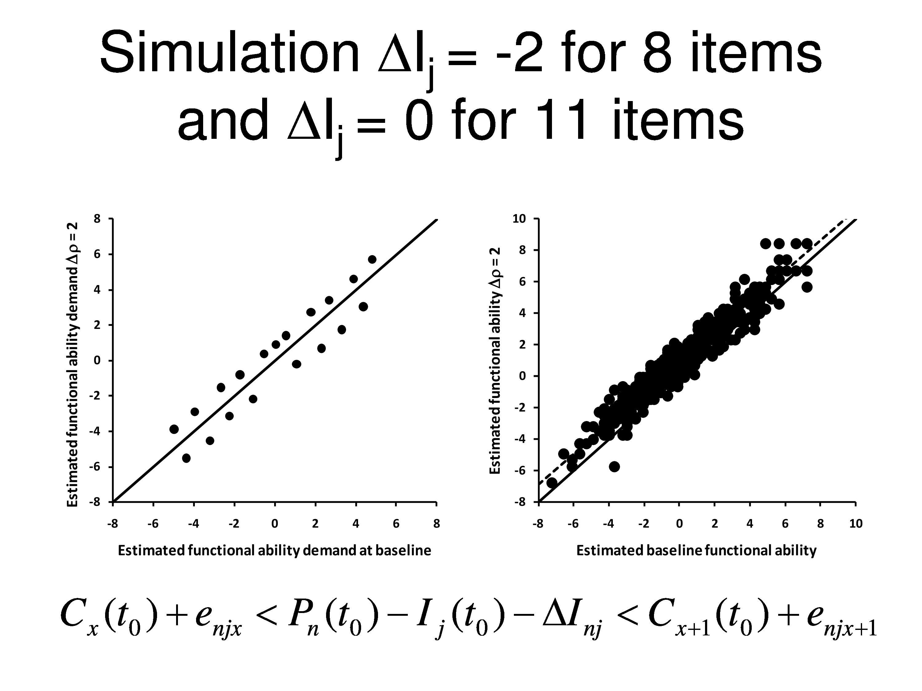
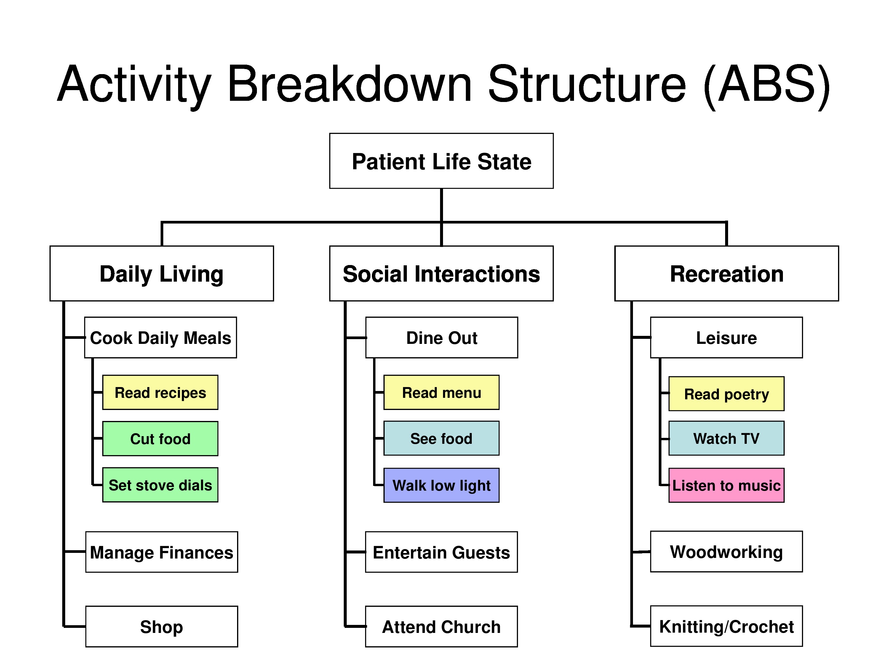
Now, out of the 19 items we’re going to change 8 of them by 2 logits. We’re going to decrease their difficulty by two logits and the other 11 items we’re not going to do anything to, we’ll keep them the same.
You may ask how is it we can change an item? How you might change an item in my field, you’re asking all these questions about activities you can do, we tackle them an activity at a time. You can’t read a newspaper, we provide you with a magnifier. You might be able to read the newspaper but you can’t read anything else with it, so that magnifier is just targeted to that one thing. Any time you’re treating a symptom that’s one of your items. When you set goals, like in goal attainment scaling, you’re treating things to achieve those goals. And you’re ignoring other things, they’re not changing.
You can end up getting item specific changes in your outcomes as a result of targeted interventions. Whether you’re working towards goals or working towards interventions that are very task specific and like accommodations or assistive equipment, things like that.
So now when we compare baseline item measures to post intervention item measures, we find that 11 items look a little bit above the line, 8 of the items had decreased by 2 logits a little bit below the line, but actually what’s happening here is that when WINSTEPS calculates item measures it takes the average of all the items and calls that zero. So when it does that then you end up straddling the line rather than the items you didn’t change being on the line. Because the average changed.
What we’ll see here is after doing that, we get a change in the person measure. There’s a very small change in the person measure, but it’s reliable, it’s about 9/10 of a logit, and that’s the dotted line that goes through the data.
What’s interesting is if you remove the 11 items that didn’t change, and we only leave the 8 items in when we run it through WINSTEPS, we delete the items that didn’t change. Then we see the person measures actually go up more.
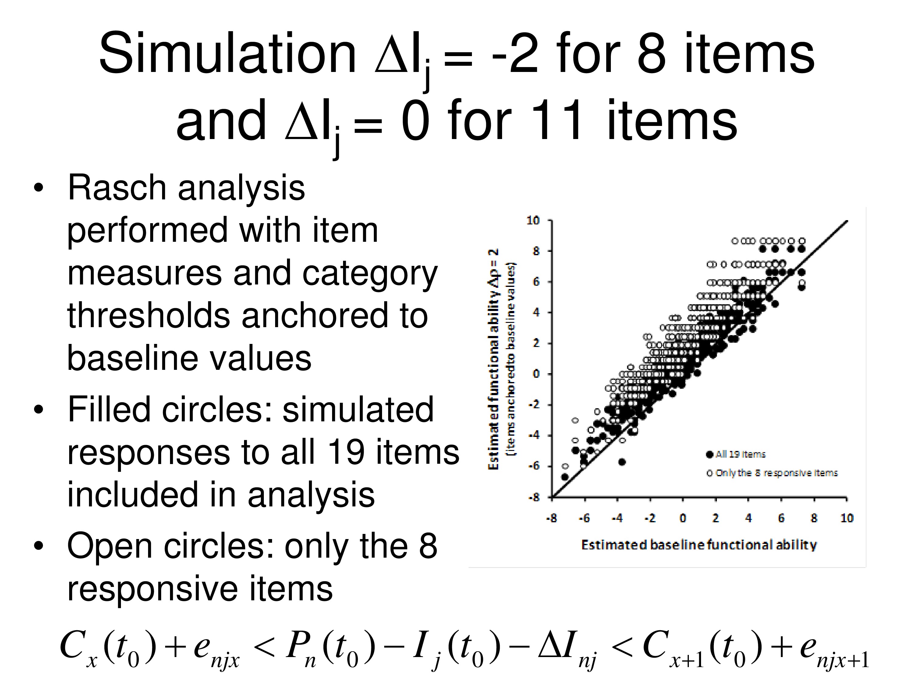
What we’re doing here is we are taking one additional step. We’re anchoring the item measures to the baseline values, which is what often is done when you’re looking at outcome steps. And we’re anchoring the category thresholds to the baseline values. And so the black dots are the person measures with all 19 items in there, but all the measures anchored. The open circles are the person measures with only the 8 items that changed and the other 11 items being deleted, still using the same anchoring. So you’re seeing a change in the person measure.
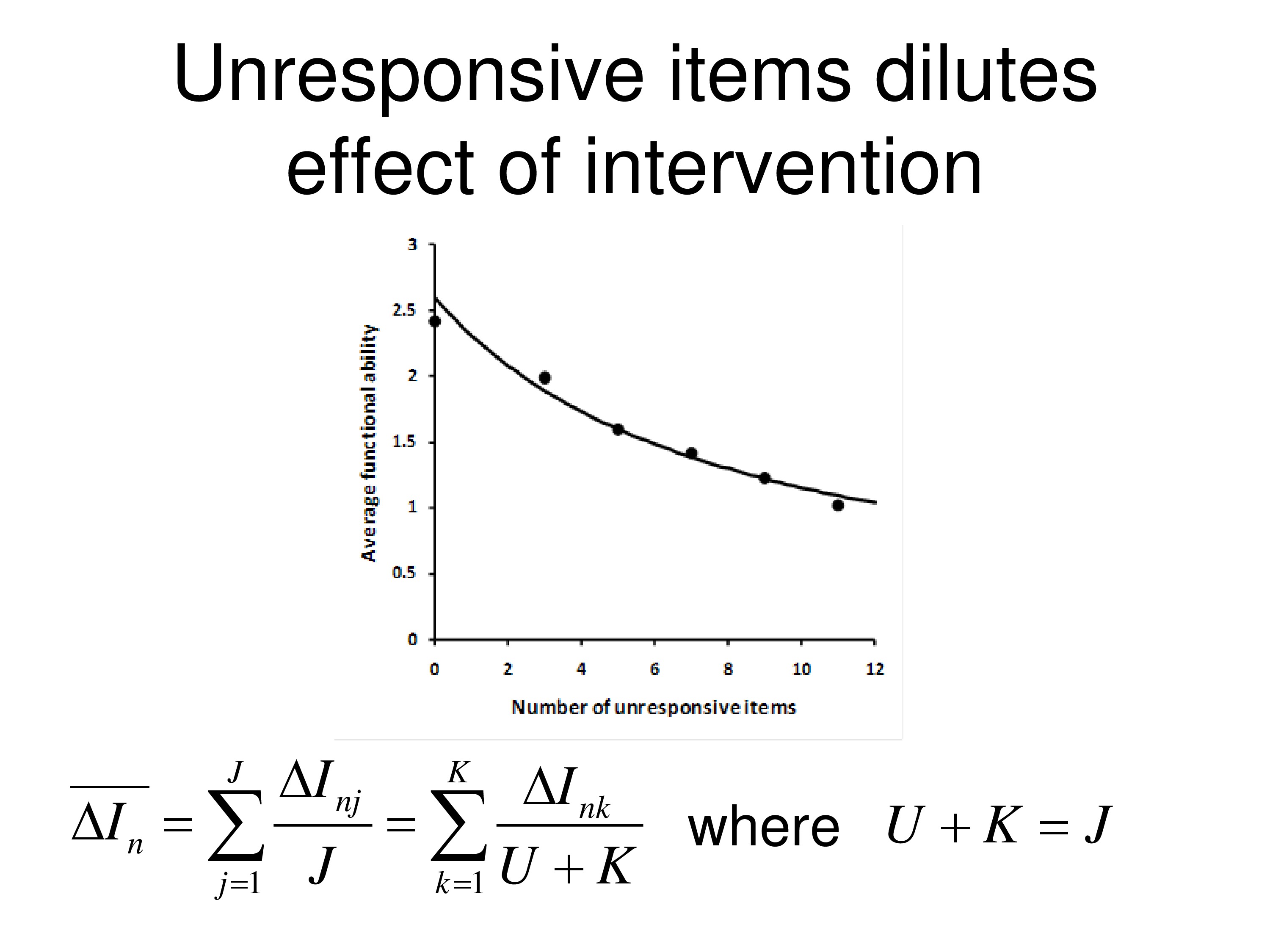
Well, if we go back to our average change in item measures, with this concept of average functional reserve, what we find out is if we’re going over j items, and j in this case if we’re 19, all 19 items, we can think of j as made up of 2 numbers. U is the unresponsive items, so there are 11 of those. K is the responsive items, there are 8 of those.
And we’re taking the average here over just the K items that they’re responsive. Now that’s legitimate because ΔI is zero for the ones that are unresponsive, so if you include them in the average or don’t include them in the average you get the same average.
But what you’ll notice, the dots on the graph, is the average change in the person measure from this, as we add more unresponsive items. So the first dot, we don’t have any unresponsive items, that’s just the 8 that responded. Second dot is that we have, I think, 2 unresponsive items included, just chosen at random. The third dot is 4 unresponsive and so on. And you can see that study drop in the person measure as you include more unresponsive items in with the items that changed. And the curve drawn through the data is from this equation. So it’s just simply person measure drops as you increase the denominator.
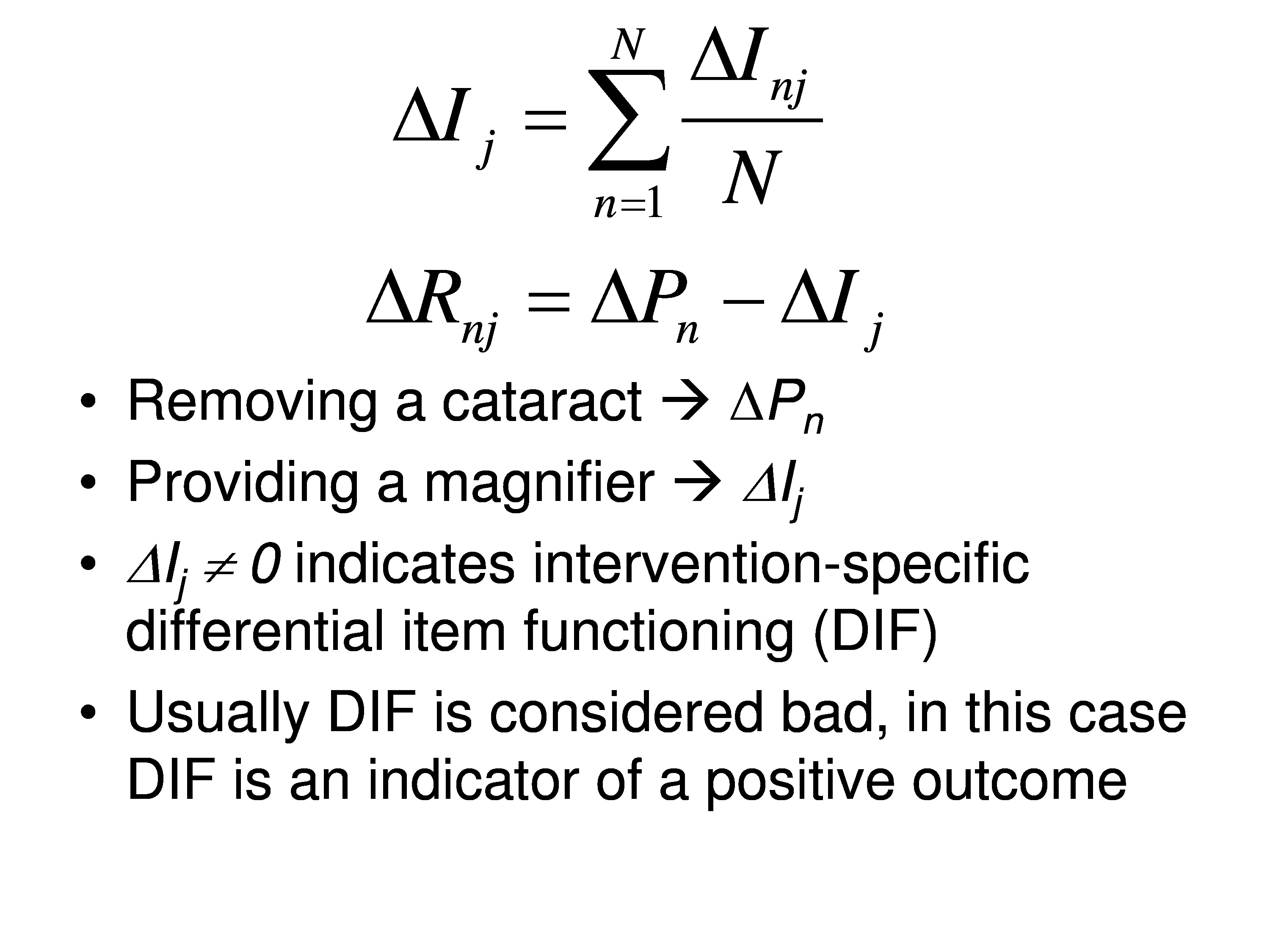
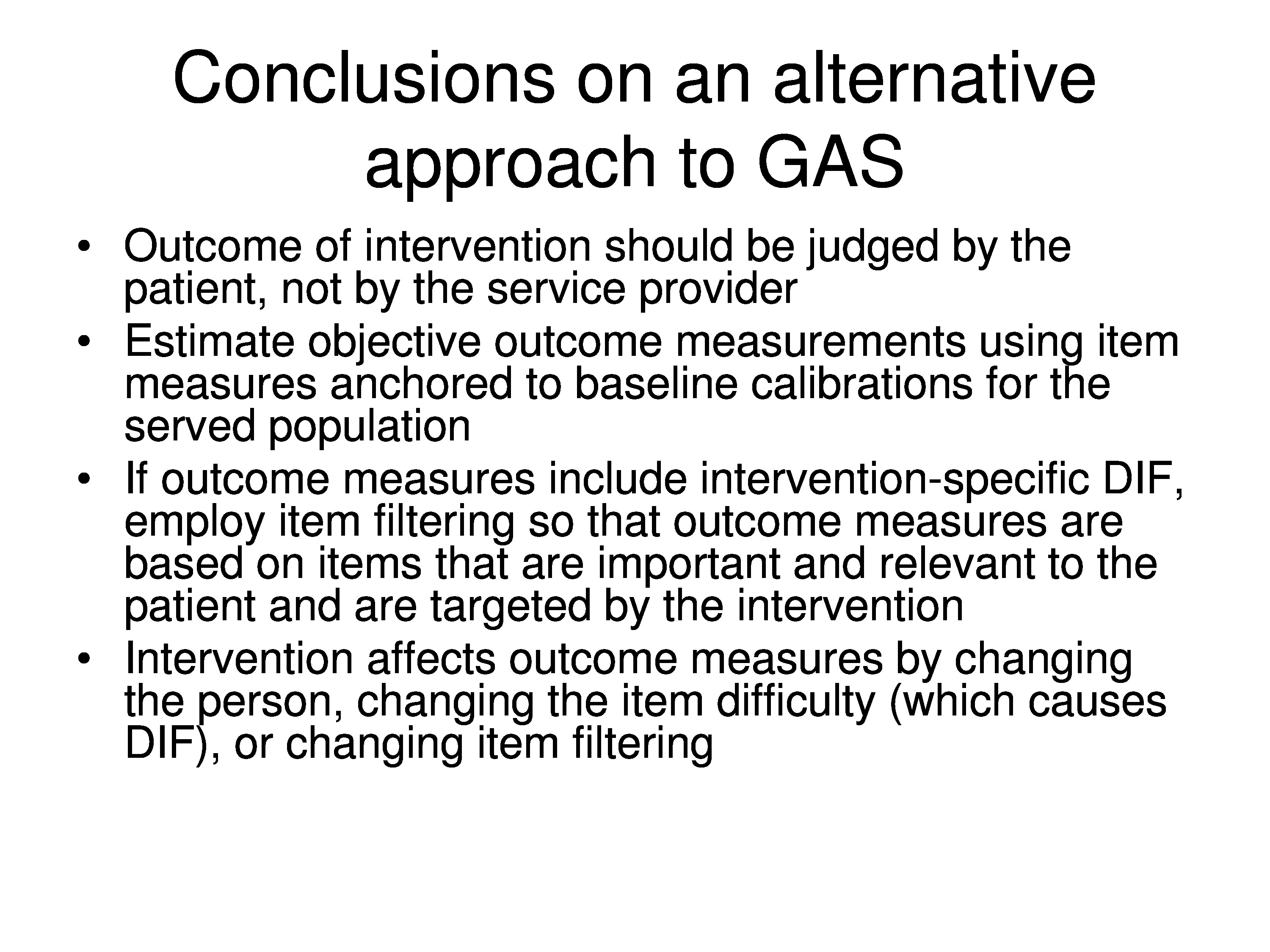
So in my field how you might change a person measure is remove a cataract. How you might change an item measure is provide them with a specific magnifier. And if the change in the item measure is not zero that indicates intervention-specific differential item functioning.
Usually DIF is considered bad, but in our case DIF is an indicator of a positive outcome. And same with goal attainment scaling, it’s an indicator of a positive outcome. So you want DIF, but you’ve got to be able to manage it and understand what’s going on.
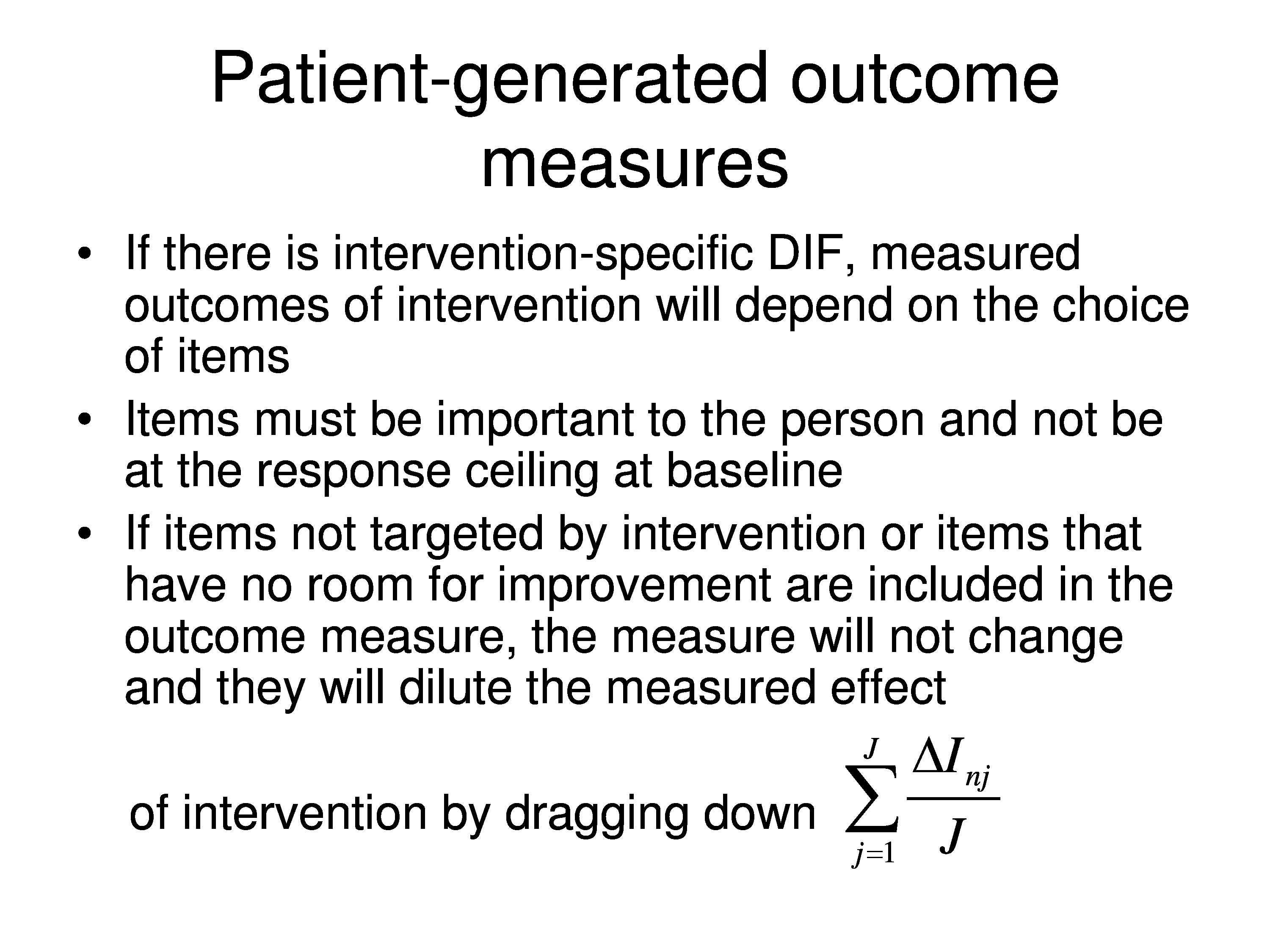
So if you use a fixed item questionnaire you might have a lot of items in there that you don’t address. And if you’re targeting items — setting them up as goals, you may be diluting your effect by including unresponsive items.
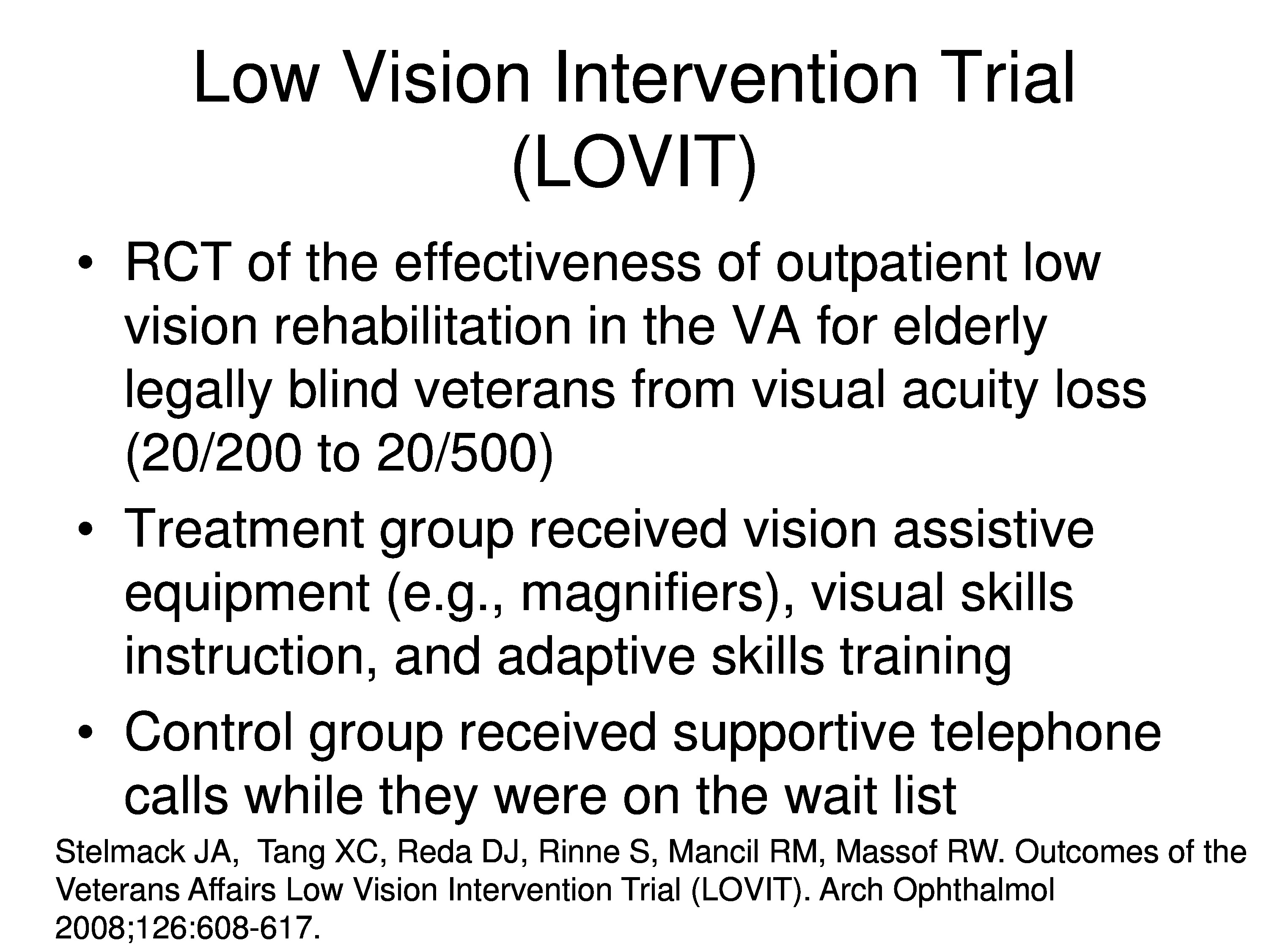
Just to show you that it’s real, that this comes out, we did a clinical trial called the low vision intervention trial at the Hines and Salisbury VAs, and they’re legally blind veterans that participated. And the treatment group got the full board low vision rehabilitation with assistive devices and everything else they need, and the control group got called every now and then and asked “how ya doing?” They were actually on the wait list to get into the blind rehab center, which gave us at least a year to finish what we we’re doing before they got their appointment to get in.

We used a 48 fixed item questionnaire. One thing with the VA BRC is that it’s kind of a one-size-fits-all program. If you’ve never cooked in your life, you have no interest in cooking, by the time you get out of the blind rehab center you’ll be the cook in the family. So the fixed item questionnaire is kind of appropriate for the VA and this one was tailored to the VA program. And the person measures are estimated from Rasch analysis by anchoring the items as we talked about before.

And this is the outcome in terms of person measure estimates. The blue is the distribution of baseline values before rehabilitation for the treatment group. And the red is the distribution of follow-up values, post rehabilitation values for that same group of patients. And I don’t have a graph of the control group, but they didn’t change. I’ll show you that in a minute and some other things. That was for reading, the one I just showed you was for reading measures.
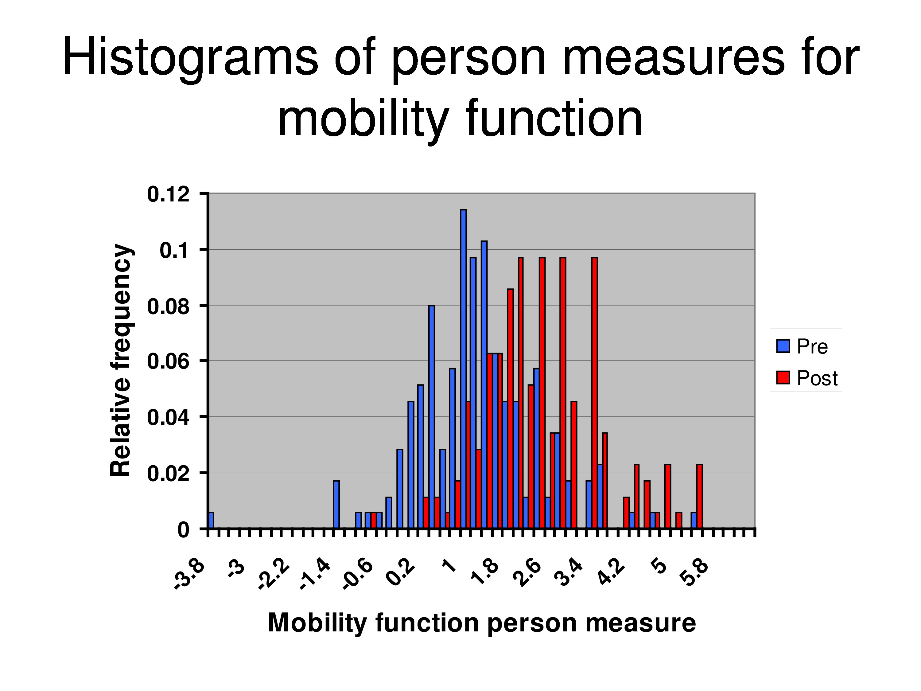
And this is for mobility. So the treatment effect was smaller for mobility.
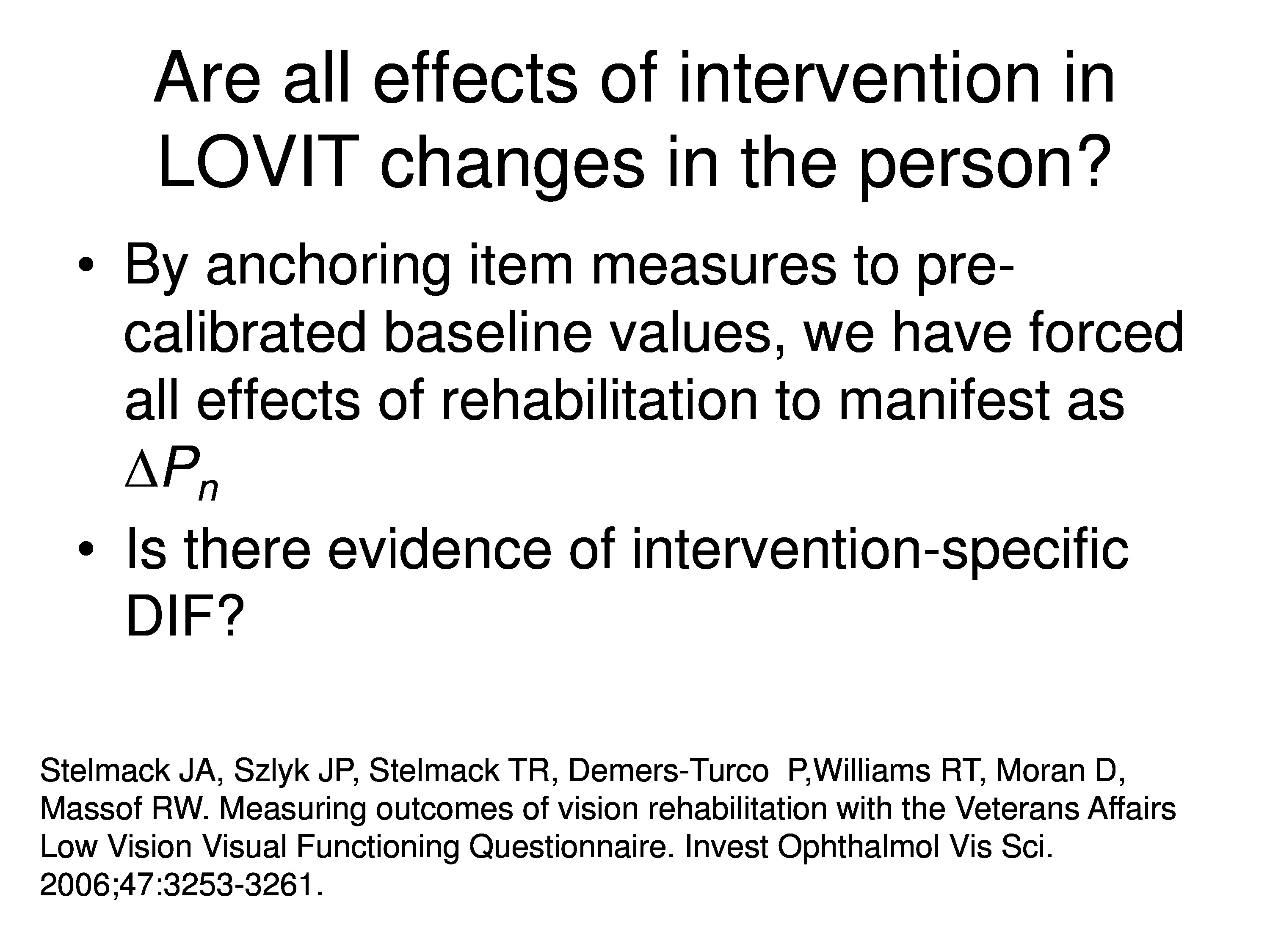
But now what we’ve done because we’ve anchored the items, we forced all the facts of rehabilitation manifest as a change of the person measure. And the question is then: Is there evidence of intervention-specific DIF?
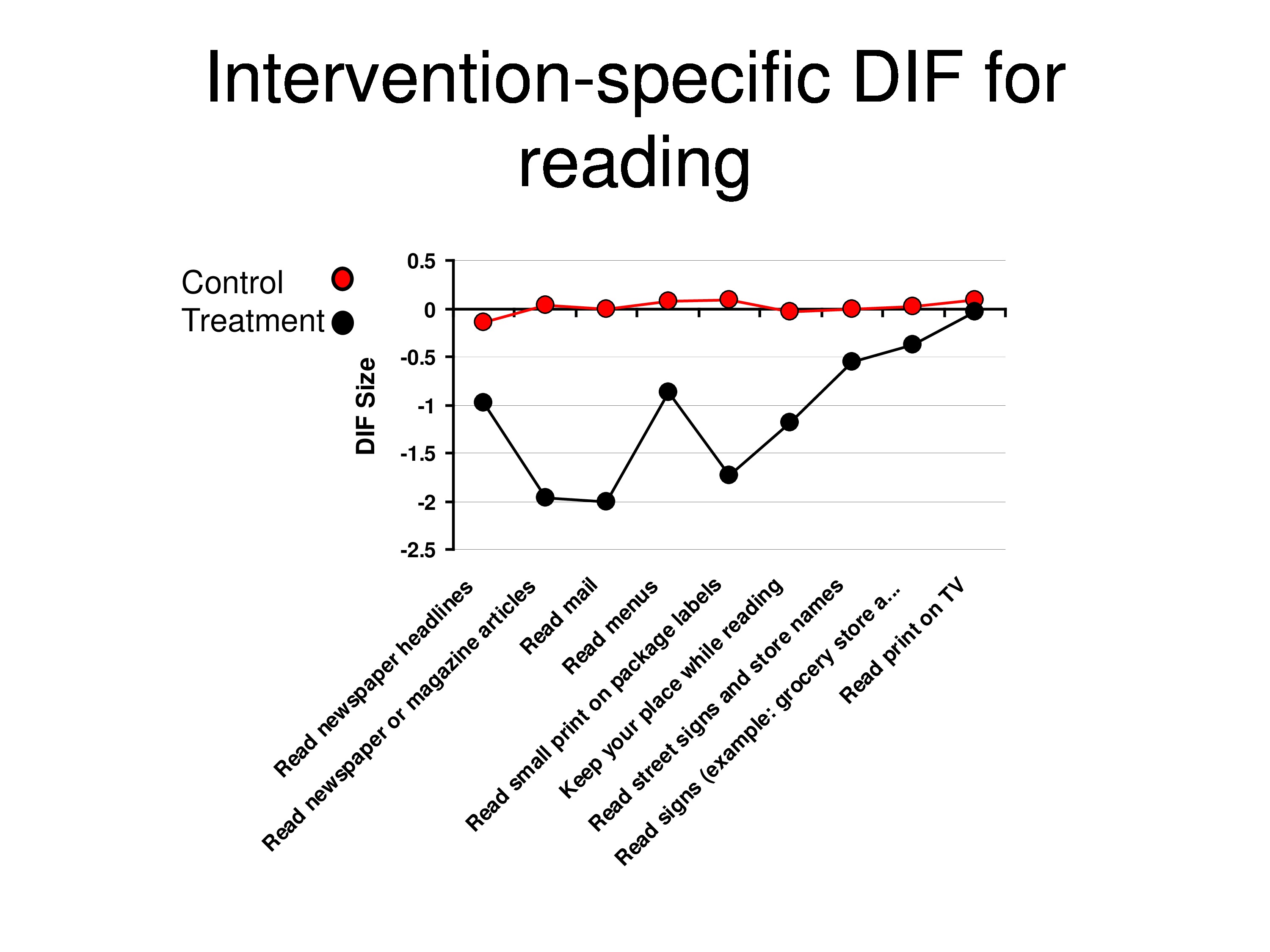
And so what we’re looking at here is relative to baseline calibrations. What is the differential item functioning post at the follow-up for the control group and for the treatment group? And what we’re seeing is that each point is a different item, not in any particular order. And that the red shows no change in items over time, but the black is showing you that there are bigger changes for some items then for others. And that’s for the reading items.
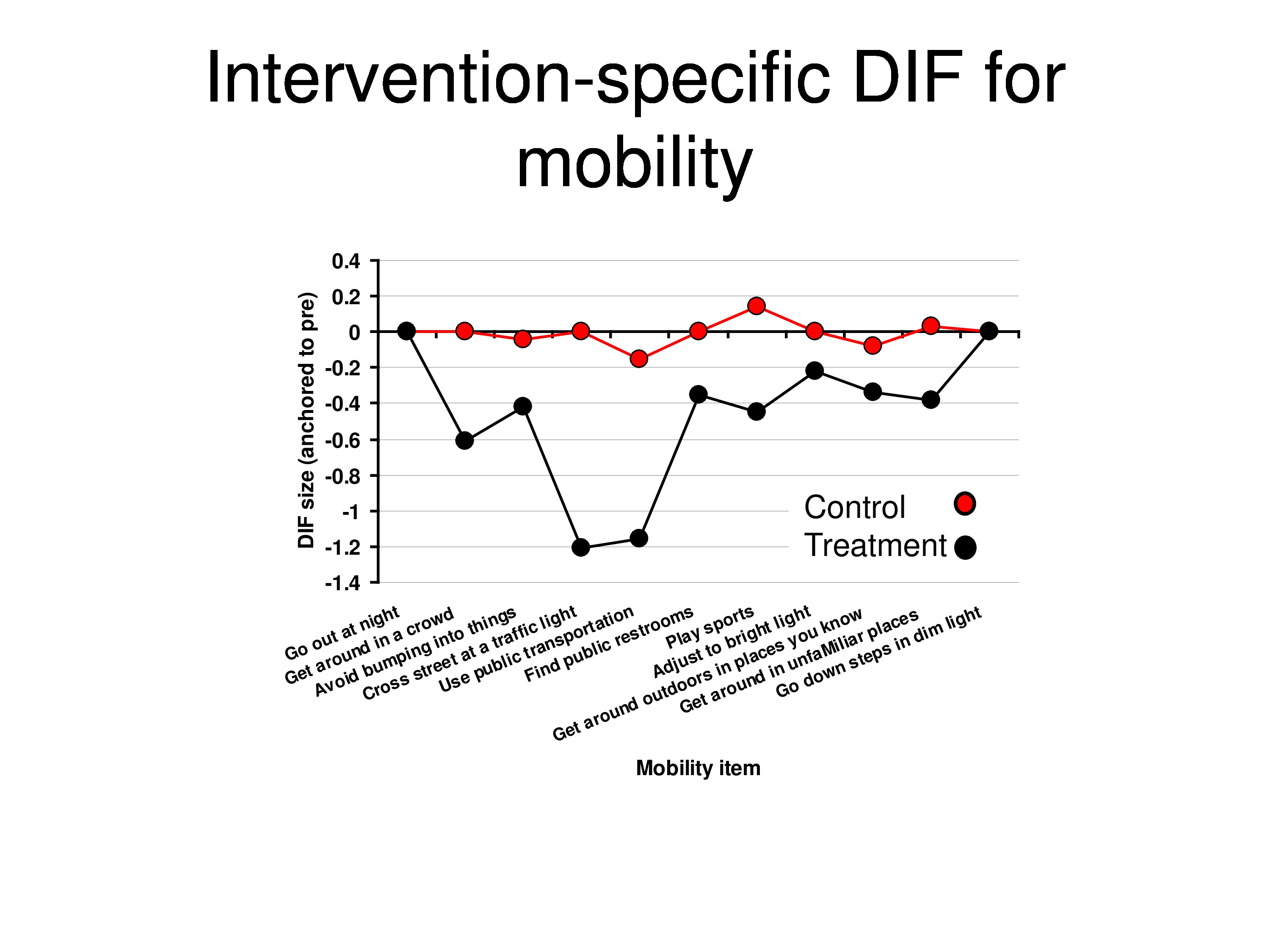
This is for the mobility items. Same story. So we are getting evidence of differential item function.
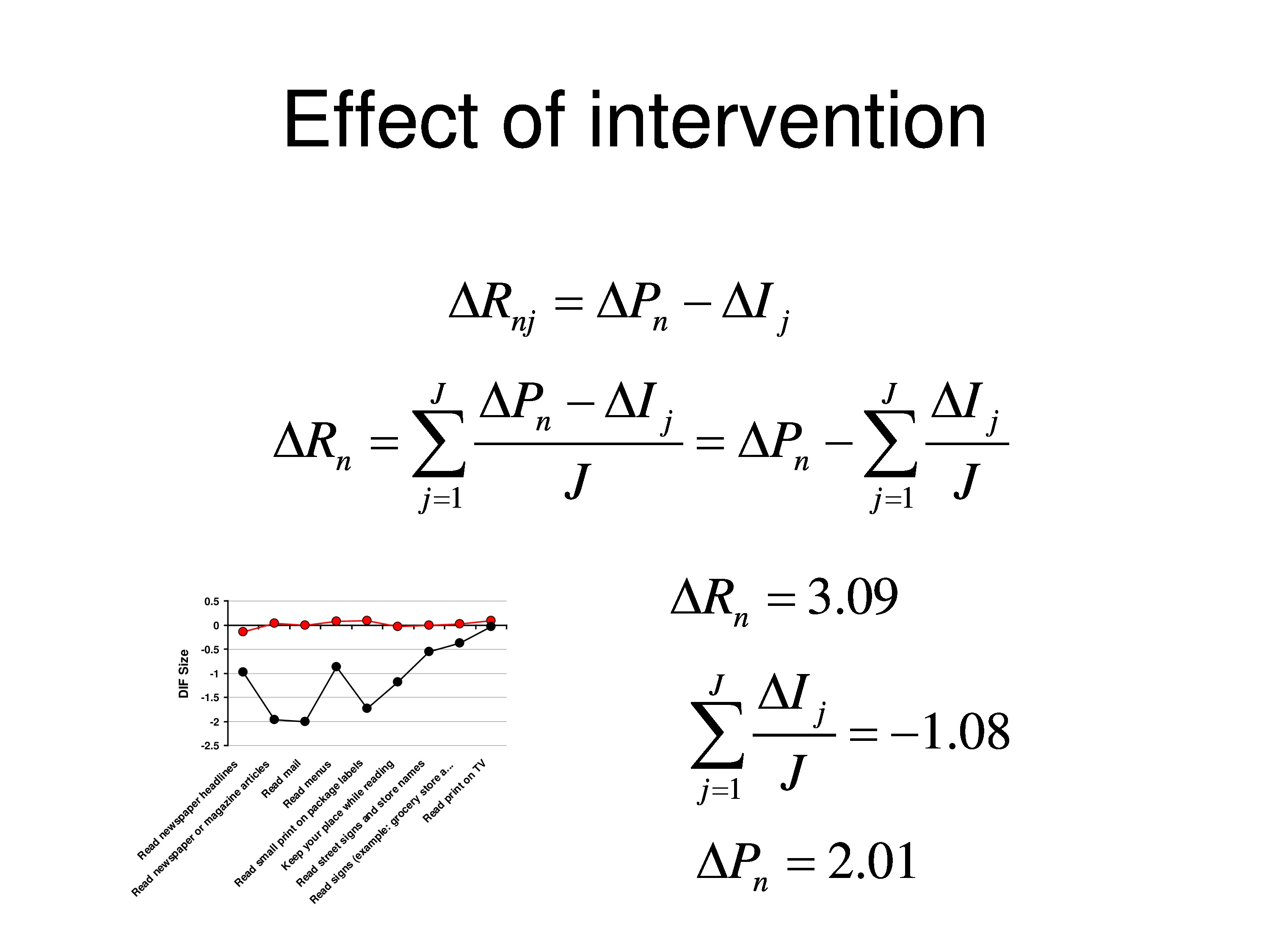
And so we can calculate what the change in functional reserve was on average for this group, and it was about 3 logits. And using the DIF analysis we can estimate what the average DIF was, and it’s about 1 logit, that it got easier.
Which means that the underlying person measure what’s common to all the items, I mean, they might have all been DIF, but if they all fall by 2 logits, which is the ΔP here, we would assign that to the person because we have no way of sorting out which is items, which is person. And then when we subtract that, you notice the last item goes up to baseline, and what’s left over is the DIF relative to that item. So we end up with this effect.
Final Thoughts
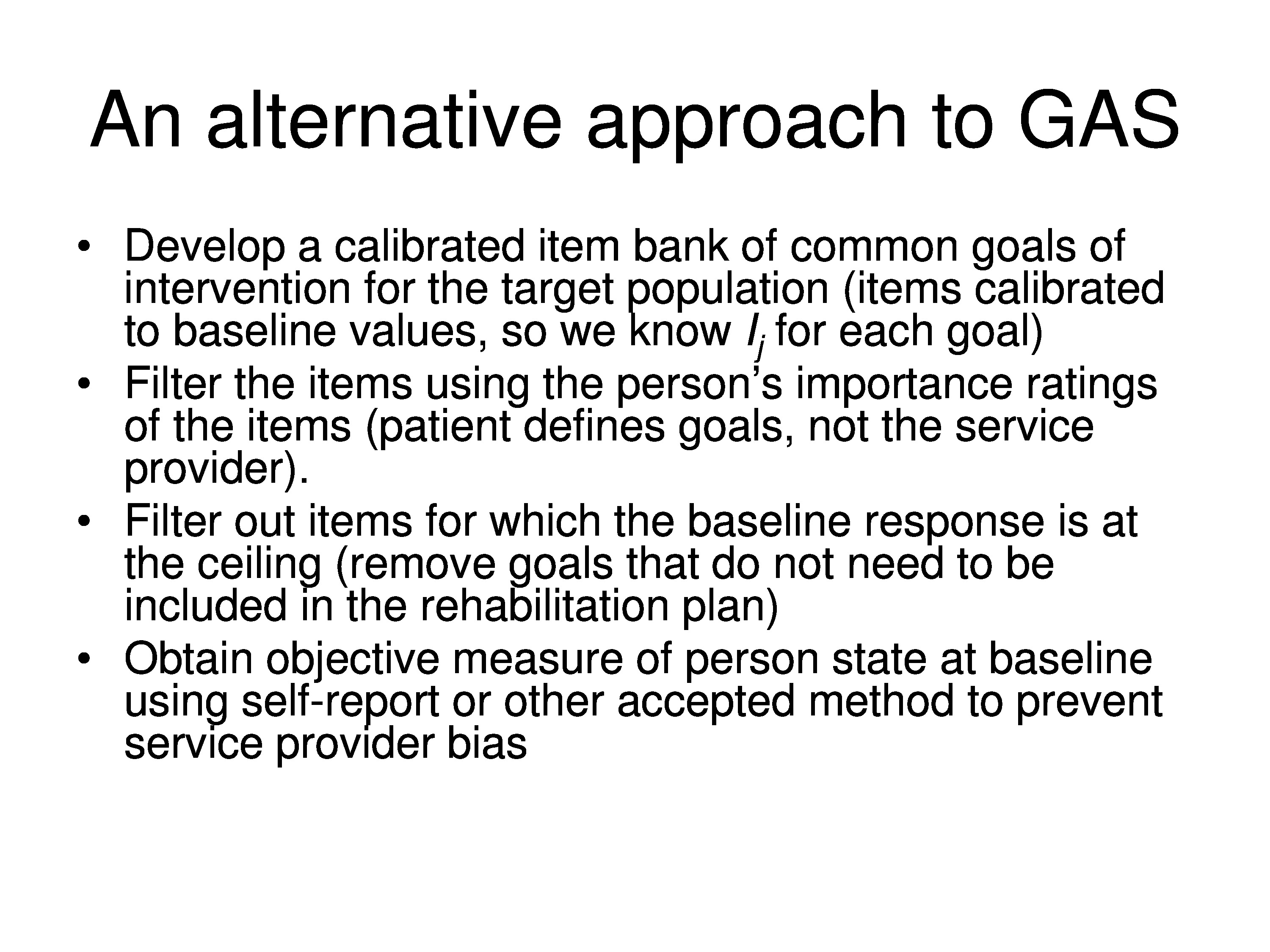
Let me just finish by saying that the way we have to modify the GAS is to take into consideration, first of all we have to anchor our items. We really should work from an item bank — not a matter of working from a floating origin. If there is a standard set of goals in your field, these goals should all be calibrated, which most likely would be items.
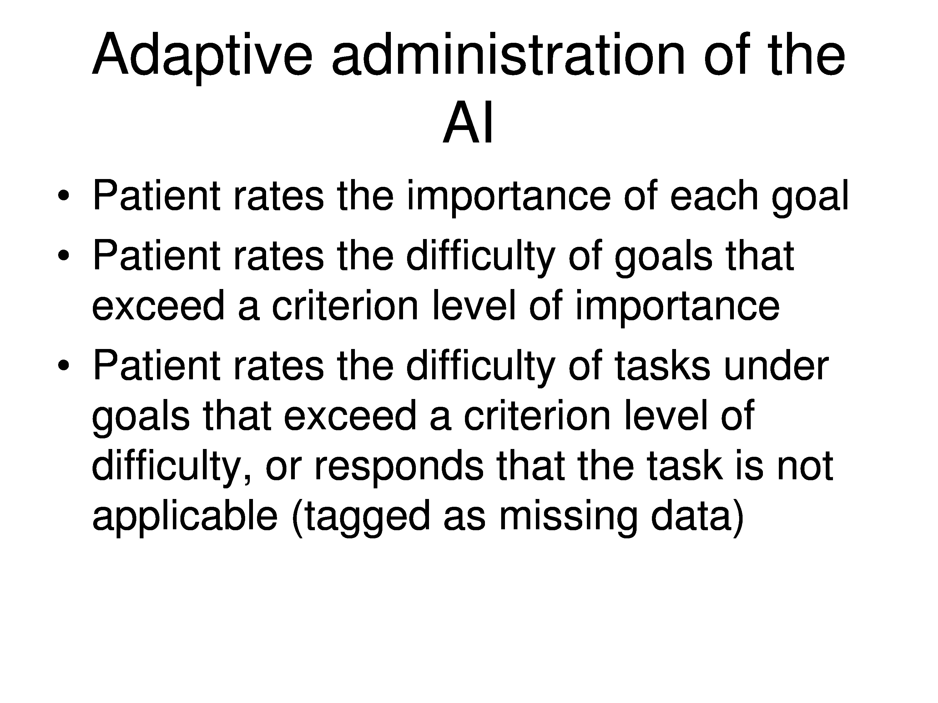
And whether we have the therapist do the rating, or the patient do the rating, or some combination of the two are doing ratings, and we’re estimating perimeters from that, the idea is to judge the outcome based on the treatment. So if a patient says an item is not important or it’s not applicable or it’s not difficult, you’re not going to address it with your therapy. Keeping it in the assessment can only lower the effect.
So then anchoring items to the baseline values of what’s left, and really the question would be, for goal attainment scaling, you only want to assess those items that represent goals. Now there are exceptions to that. If you’re not doing goal targeted interventions. If I change one thing it’s going to change their lives all the way across the board, but you know, I won’t quarrel with those people, but for a lot of rehab we’re very much oriented for very specific targets.
And the bottom line, it doesn’t make a great deal of difference which of these many models you use. They all pretty much produce the same answers within tolerance, but there are theoretical considerations on all of these things, and I would urge you all to kind of get down to the weeds with the rest of us and learn about what your computer program is doing when it’s estimating these parameters, because a lot assumptions are being made that we’re not even talking about at these meetings. And if you knew what they were you would probably throw up your hands and say, why am I doing this?
So be cautious in terms of the models you’re using. It’s important, I think the next step in the development of the field is to understand these models and make sure that the models represent what you believe to be going on and they represent what you’re trying to do. You’re not simply generating numbers wondering why you’re getting all this variability.
Most scientist are kids – go back to being that skeptical kid. You know, when somebody tells you about their great model it’s probably wrong. All models are wrong. So find out what’s wrong with it and don’t be satisfied until you do find out what is wrong with it. All these models are very absolute in their assumptions, and it’s kind of like, what are you willing to accept? What’s the most reasonable?
So you want to, at the very least, understand the assumptions. You don’t necessarily have to get down and do the computations, but understand what assumptions are going into these models, and do they fit your situation.
Like the graded response model is based on a physics model. The graded response model has a very strong assumption in it, and that strong assumption is that the category thresholds are fixed, they do not vary between people. Do you believe that? If you don’t why are you using it?
Rasch model has a very strong assumption, it says all variability comes in through the category thresholds, that there is no variability in the item interpretation. Item interpretation variability introduces correlations that the Rasch model can’t live with. If you say, well, that’s fine, that’s probably the major source of variability between people, then use the Rasch model.
Other models, each model as it adds more and more parameters can explain more and more things. So if you see a model laden with parameters coming in, and some of the models we heard today do a very good job of fitting the data at hand, but they become sample specific. They end up simulating what you have and not really necessarily explaining anything. But, you end up with a parallel and kind of description of what the equations are doing and you forget this model. That’s a flag that you should be skeptical about: Why do need so many parameters in order to explain what’s going on.
Questions and Discussion
Question: You mentioned that if you delete the item where no change was found, that the person functionality increased. Does that mean that zero change was found? Do you include the items if even a moderate change was there? And was there a time variable in there to allow for change over a certain point?
Well, it depends on what you’re trying to assess. If what you want to know is, where is this person in relation to where they were at baseline? Then you maybe want to leave the items in.
On the other hand, if what you want to know is, what did my treatment do relative to the goals I set? Well, if you have somebody who comes in and has fairly modest goals, that you know, most things are okay but there’s just a couple things we’ve got to fix, you could hit a homerun. But all those other items that don’t change because they weren’t difficult to begin with, they will wash out your effect. You’re not going to see much of an effect. If you’re designing a big expensive clinical trial to look for this and you know, you’re going to find that it’s going to be down in the noise.
On the other hand, you can make relatively trivial changes: there are 100 things they should be able to do and you’re only going to work on two of them and so you throw out 98 of them. You could have a huge effect and just exaggerate the magnitude of what you’re doing. So there’s a certain amount of auditing that has to be done in terms of making it clear of what it is you’re trying to describe. A change in what?
It’s a complicated story, and it lends itself to abuse and cherry picking and doing things to inflate the numbers once you understand how to do it, but it’s probably better that you know if you’re doing it, to know that is what’s happening as opposed to just kind of going ahead and administering an instrument and then wondering why you’re not seeing much of a change as a result of your treatment.
And we’ve seen that in low vision. The Lovett study is getting huge effects, 2, 3 logits, yet the rest of the world is getting effects on the side of just 3/10 of a logit, presumably doing the same things, but using very different instruments not designed for the intervention and so on.
Question: Could you say a few words about the implications of treatment-induced DIF for computerized adaptive testing?
Another part of this paper which is going to be coming out is looking at the effects of these assumptions on CAT. Remember that CAT uses anchored items. So you calibrate all the items, they have fixed values. You calibrate the category thresholds, they all have fixed values. Now you’re going through and estimating person measures on a person-by-person basis using these fixed items and an algorithm that choses items based on your previous responses.
If the item changed, when you go back into the bank to pull out the next item, you’re going on the basis of the item measure. You’re not going on the basis of any other information except how they responded to the one you just gave them. So as a result, you’ll find yourself kind of see-sawing then you get into a hysteresis that has trouble converging on a solution, because you’re pulling out items that might have changed. So the items aren’t where you thought they should be. And then what we found in simulations, and it depends on how many items you have that changed and how many are in your pool and things like that, but in the simulations we found that it had trouble converging and then all the sudden it would start to converge, but it would converge on the baseline value. So it would converge at no effect.
And so to use CAT as an outcome measure, before you believe it, I think you have to say, is there differential item functioning as a result of my intervention? And you might want to take a look at that before you jump in and use a CAT.
And CAT already knows that you shouldn’t have DIF in there because they correct for that when they know its present, and you know, in PROMIS study DIF is a big important issue. But usually the kind of DIF they’re looking for is like gender or comorbidities or some other things.
References
Kiresuk, T. J. & Sherman, M. R. (1968). Goal attainment scaling: A general method for evaluating comprehensive community mental health programs. Community Mental Health Journal, 4(6), 443–453 [Article] [PubMed]
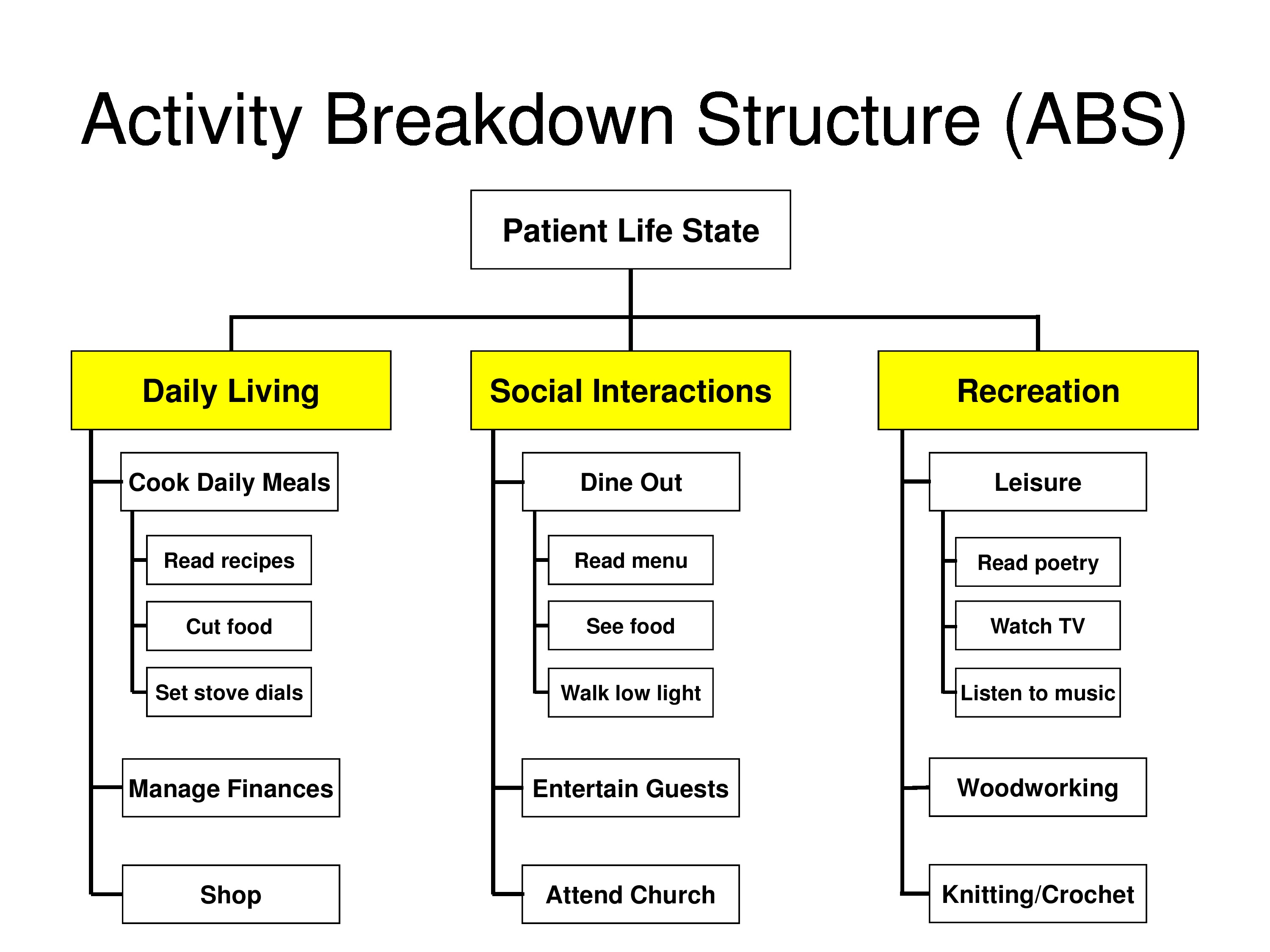
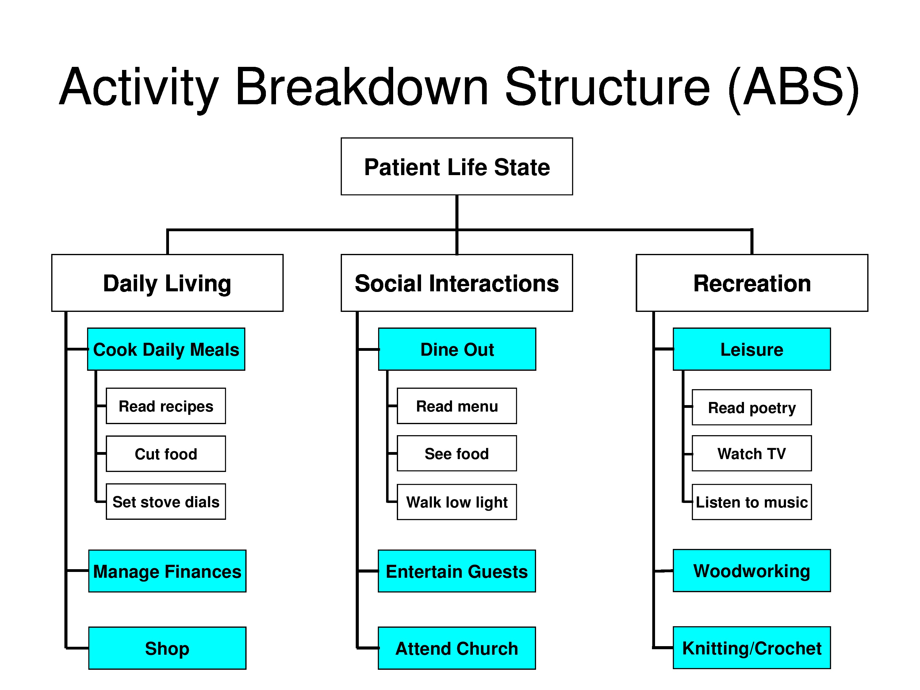
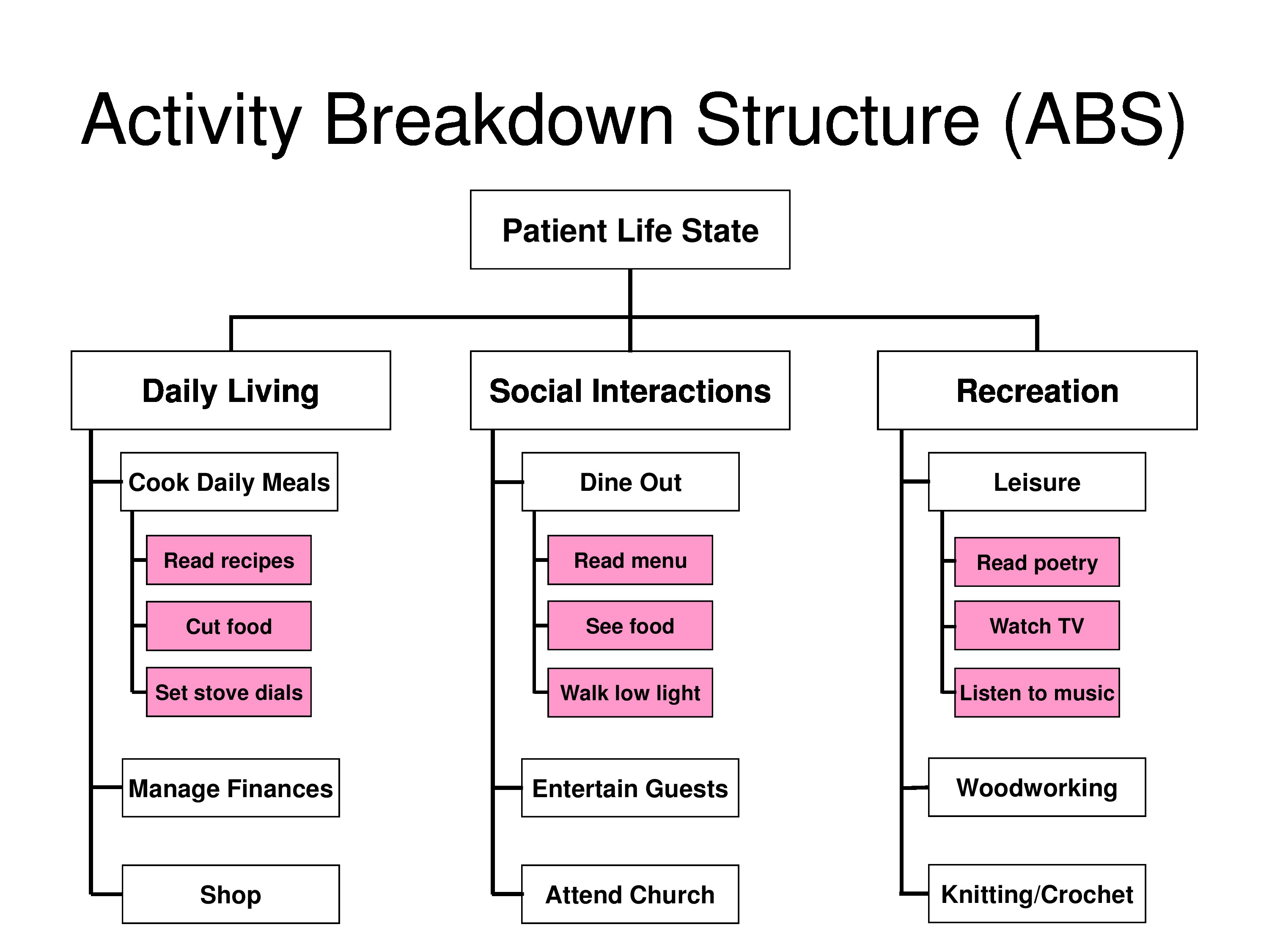
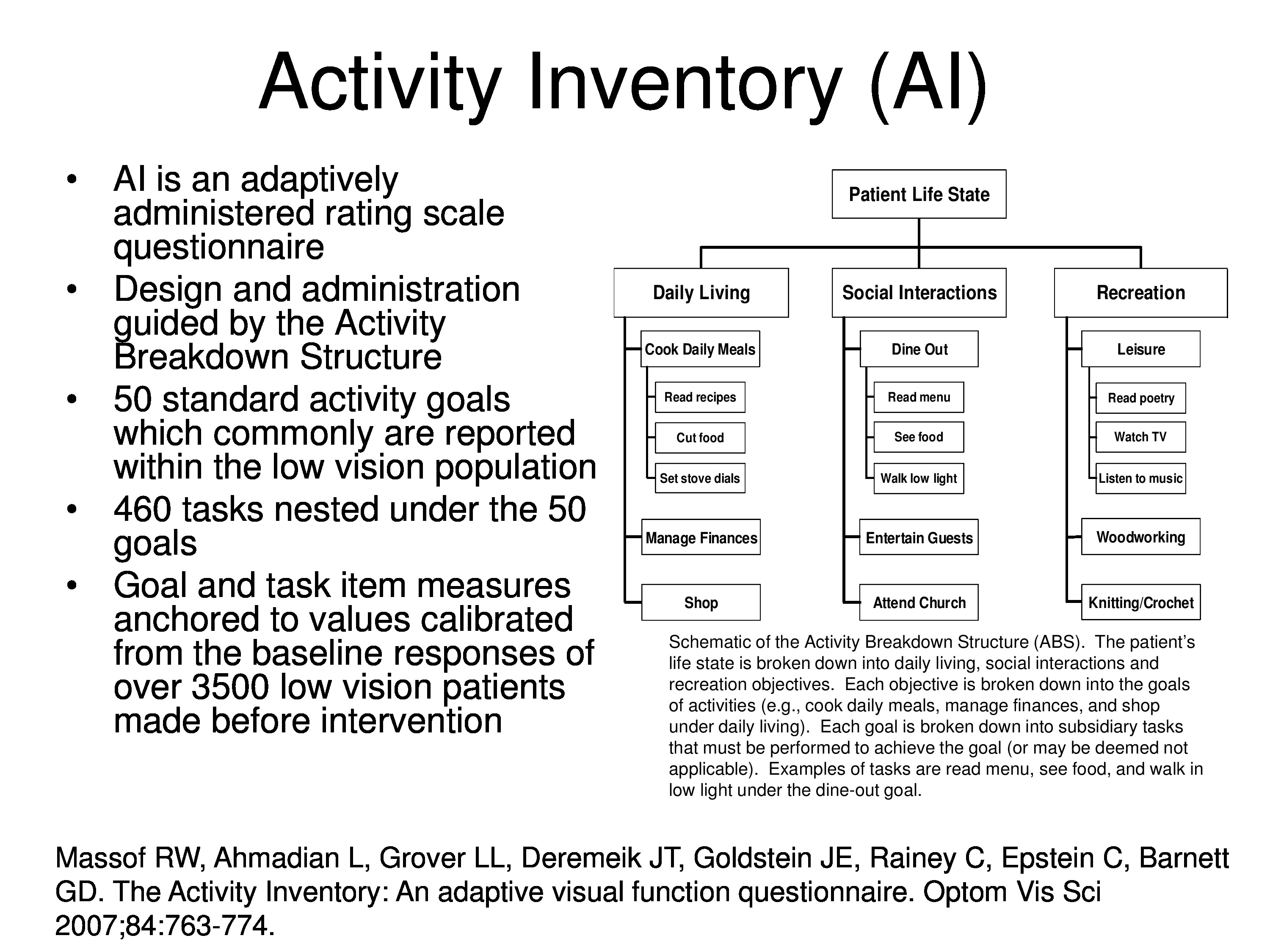
Massof, R. W., Ahmadian, L., Grover, L. L., Deremeik, J. T., Goldstein, J. E., Rainey, C., Epstein, C. & Barnett, G. D. (2007). The activity inventory: An adaptive visual function questionnaire. Optometry & Vision Science, 84(8), 763–774
Stelmack, J. A., Szlyk, J. P., Stelmack, T. R., Demers-Turco, P., Williams, R. T. & Massof, R. W. (2004). Psychometric properties of the veterans affairs low-vision visual functioning questionnaire. Investigative Ophthalmology & Visual Science, 45(11), 3919–3928 [Article] [PubMed]
Stelmack, J. A., Szlyk, J. P., Stelmack, T. R., Demers-Turco, P., Williams, R. T. & Massof, R. W. (2006). Measuring outcomes of vision rehabilitation with the veterans affairs low vision visual functioning questionnaire. Investigative Ophthalmology & Visual Science, 47(8), 3253–3261 [Article] [PubMed]
Stelmack, J. A., Tang, X. C., Reda, D. J., Rinne, S., Mancil, R. M. & Massof, R. W. (2008). Outcomes of the veterans affairs low vision intervention trial (LOVIT). Archives of Ophthalmology, 126(5), 608–617 [Article] [PubMed]
Turner-Stokes, L. (2009). Goal attainment scaling (GAS) in rehabilitation: A practical guide. Clinical Rehabilitation, 23(4), 362–370 [Article] [PubMed]
Appendix: Additional Slides
Slides included in the final presentation file, which the presenter did not have enough time to cover during the session.